Overview
orbital-radar.py (Pfitzenmaier et al., 2024 - in preparation) is a Python package which transforms suborbital profiling cloud radar data (ground-based or air-born) into synthetical satellite cloud profiling radar (CPR). An example is the CPR of ESAs EarthCARE mission; NASA’s CloudSat mission can be simulated, too. By resampling the input data, the code mimics the CPR hardware specifications, calculates the noise-free CPR reflectivity and Doppler velocity fields, and, in an additional step, adds the system’s characteristic noise and errors. Using this optical-radar.py generates synthetic L1 satellite CPR data files.
The code can handle several cloud radar data input formats. Therefore, it is possible to transform large ground-based radar data sets from networks such as ACTRIS (ACTRIS data portal) or ARM (ARM web page) with suborbital-radar.py. So statistically robust data sets are generated, which can be used for algorithm testing, Cal/Val method development, or testing new satellite configurations.
1. Supported data formats:
To support a broad user community, the code supports the following input formats for radar data:
Generic Earth Observation Metadata Standard (GEOMS) from ESA and NASA (GEOMS information link)
Cloudnet categorisation file; Cloud Remote Sensing format from ACTRIS (ACTRIS data portal)
ARM radar data format (ARM web page)
RPG 94 GHz AC3 data format based on University of Cologne radar processing code (GitHub repository of the Matlab processing <https://github.com/igmk/w-radar>)
Air-plane: MIRAC-A data from Polar 5 (AWI, Bremerhaven, Germany)
Air-plane: RASTA data from Falcon (LACMOS, Paris, France)
2. Structure of the code:
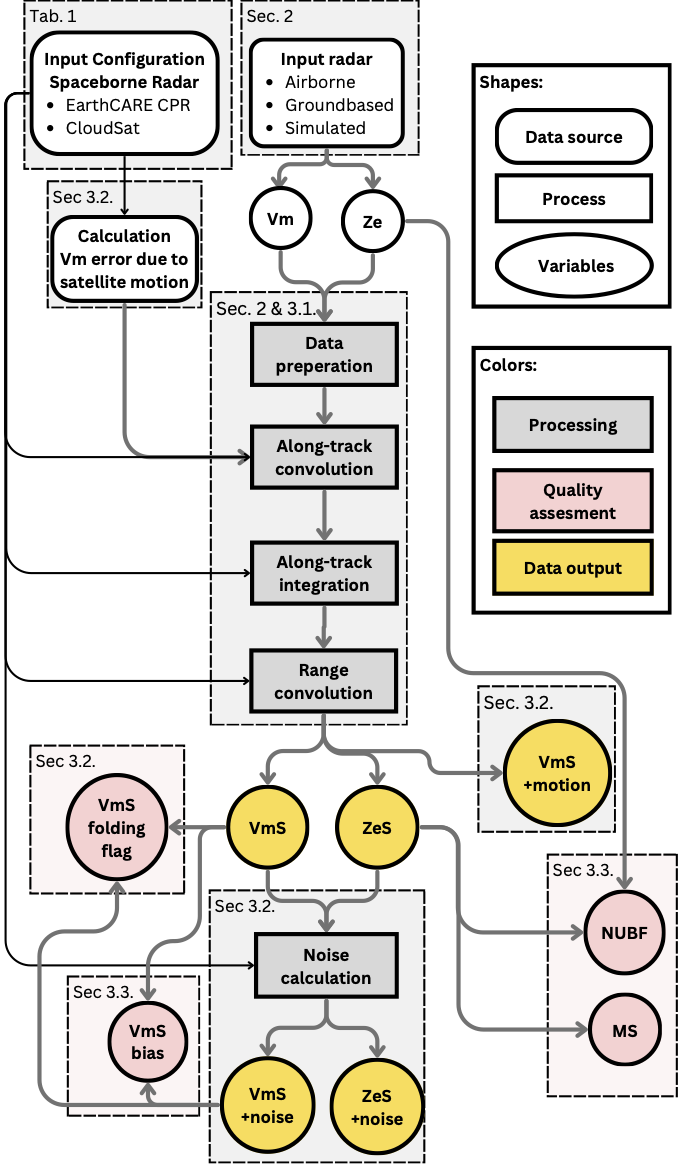
The code structure is illustrated in the flowchart.

Workflow of suborbital-radar.py .
Further explanations about the single steps of the code, parametrisations or thresholds used in the tool are presented in Pfitzenmaier et al., 2024 (in preperation)
3. Example:
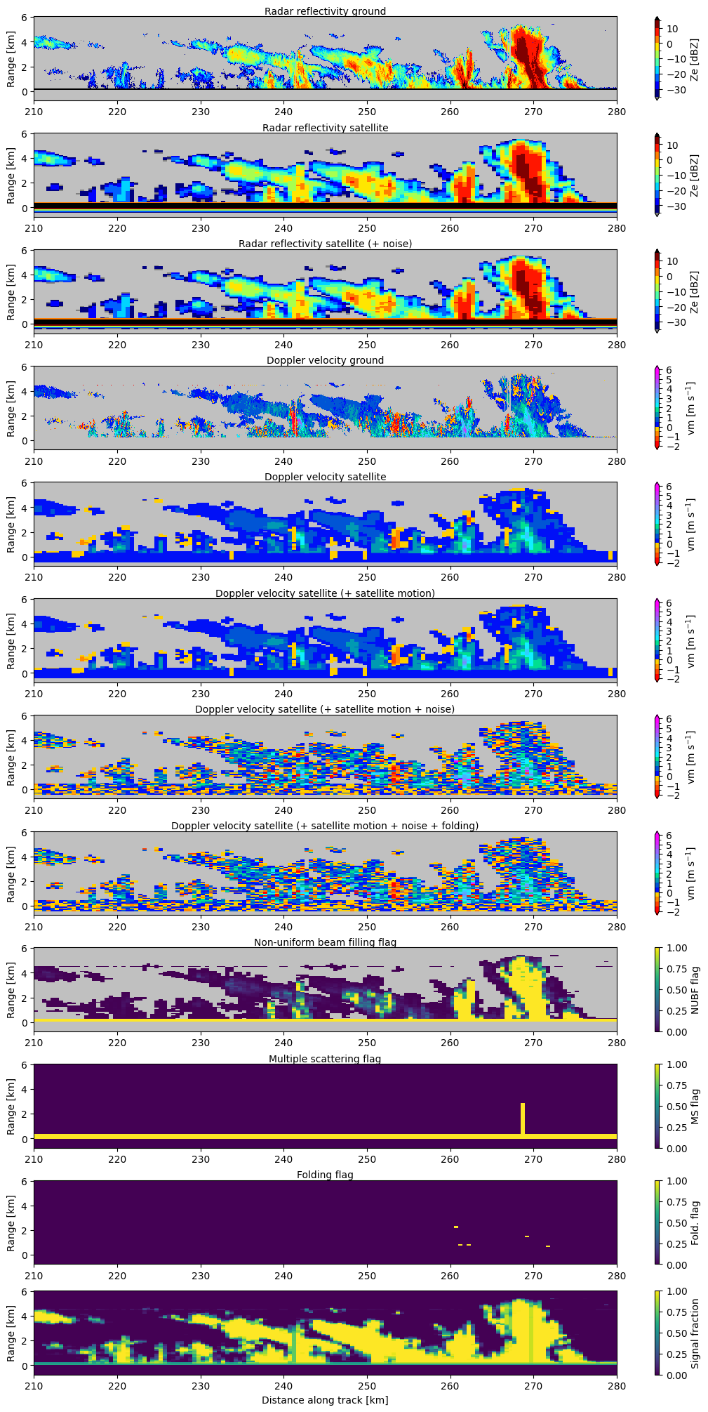
The following section shows an example data case simulated with orbital-radar.py. Simulations based on MIRAC-A measurements from the ACTRIS site JOYCE, Jülich, Germany, from 6th April 2021. The figure shows input data (first and fourth row) and all the intermediate products of the code, as well as the quality flags calculated.

Example: Synthetic EarthCARE CPR for MIRAC-A data at ACTRIS site JOYCE, Jülich, Germany, from 6th April 2021.
Bullet points explain the figure from top to bottom:
ground-based radar reflectivity (Ze) input - added synthetic ground echo and axes conversion time-axes to along-track axis and y-axis extension towards negative hights
synthetic CPR Ze field without noise - best Ze estimate from space
synthetic CPR Ze field with added noise
Ground-based radar Doppler velocity (Vm) input data in new coordinate system
synthetic CPR Vm field without noise - best Vm estimate from space
synthetic CPR Vm field with added satellite motion error
synthetic CPR Vm field with added satellite motion error and NUFB filling, Doppler spectrum broadening and random error. Velocities are not folded
synthetic CPR Vm field with all error sources added and folding applied
calculated std of Ze of the ground base data to calculate the synthetic CPR (large std(Ze) indicates large NUBF in the synthetic CPR)
Calculate the quality flag for multiple scattering (MS). 0= no MS; 1=MS in the pixels
calculated quality flag for Doppler velocity folding. 0= no Doppler velocity folding within the volume; 1= Doppler velocity folding in the volume.
calculated the expected Doppler velocity bias due to NUBF.
4. Output formats:
suborbital-radar.py provides an output formats. There will be no output mimicking the EarthCARE C-NOM format (CNOM documentation). The output option provided contains input used by and output data generated by the tool - see all output data in the schematic in Sec 2. These are the input data files (ground/air-plane truth), synthetic CPR best estimates (no noise added to the data), and the synthetic CPR data (Ze and Vm fields including noise). So the users can choose their output data file depending on their own needs.
5. Use of the Code:
To get started with ‘orbital-radar.py’ please follow the instructions in Chapter.
- Getting Started
here all additional preparations are given before the installation
Installation explaining the installation process
the provided demo.ipynb-notebook will, together with the test data sets, show you how to use the code (repository given in Chapter Getting Started)