HALO-AC3

This example demonstrated the use of ac3airborne for HALO flights during HALO-AC3.

For the instalaltion of required modules, see: https://speicherwolke.uni-leipzig.de/index.php/s/cgzrgH5nX3dxAso

If you run into problems with the code or just want to share your plots, feel free to join the ac3airborne channel on slack!

import ac3airborne
from ac3airborne.tools import flightphase
import numpy as np
import matplotlib.pyplot as plt
from matplotlib.colors import to_hex
import matplotlib.dates as mdates
from matplotlib import cm
import ipyleaflet
from ipyleaflet import Polyline, Map, basemaps, basemap_to_tiles
from ipywidgets import Layout
from simplification.cutil import simplify_coords_idx
import os
%matplotlib inline

To access the data from the cloud server easily, the credentials can saved in an environment variable of your computer (or typed in directly here).

ac3cloud_username = os.environ['AC3_USER']
ac3cloud_password = os.environ['AC3_PASSWORD']

credentials = dict(user=ac3cloud_username, password=ac3cloud_password)

Select a flight

To select a flight, specify the mission, platform and flight number in the flight_id.

mission = 'HALO-AC3'
platform = 'HALO'
flight_id = 'HALO-AC3_HALO_RF03'

Load intake catalog and flight segments

The first HALO flights are already divided into logical segments. We can check the meta data of the selected flight here.

# load intake catalog and flight segments
cat = ac3airborne.get_intake_catalog()
meta = ac3airborne.get_flight_segments()

flight = meta[mission][platform][flight_id]

list(flight)

['co-location',
 'contacts',
 'date',
 'events',
 'flight_id',
 'flight_report',
 'landing',
 'mission',
 'name',
 'platform',
 'remarks',
 'segments',
 'takeoff']

Read data of flight

Several datasets are already available on the cloud. Here we present an example for the HAMP data as well as the basic gps information.

# get list of available datasets
list(cat[mission][platform])

['BAHAMAS',
 'BACARDI',
 'DROPSONDES',
 'DROPSONDES_GRIDDED',
 'GPS_INS',
 'HAMP_KV',
 'HAMP_11990',
 'HAMP_183',
 'HAMP_MIRA',
 'KT19',
 'SMART',
 'AMSR2_SIC']

When we use caching, we do not need to download the data every time we call the script.

# local caching
kwds = {'simplecache': dict(
    cache_storage='/work/data/halo-ac3', 
    same_names=True
)}

# read hamp data
ds_hamp_kv = cat[mission][platform]['HAMP_KV'][flight_id](storage_options=kwds, **credentials).to_dask()
ds_hamp_119 = cat[mission][platform]['HAMP_11990'][flight_id](storage_options=kwds, **credentials).to_dask()
ds_hamp_183 = cat[mission][platform]['HAMP_183'][flight_id](storage_options=kwds, **credentials).to_dask()
ds_hamp_mira = cat[mission][platform]['HAMP_MIRA'][flight_id](storage_options=kwds, **credentials).to_dask()

# read gps
ds_gps_ins = cat[mission][platform]['GPS_INS'][flight_id](storage_options=kwds, **credentials).to_dask()

Plot flight on map

This map provides an overview of the flight using VIS satellite imagery and labels for every segment. The code is simply copied from here: https://igmk.github.io/how_to_ac3airborne/flight_segmentation.html

def colors(n):
    """Creates set of random colors of length n"""
    
    cmap = cm.get_cmap('gist_rainbow')
    rnd = np.random.uniform(low=0, high=1, size=n)
    cols = cmap(rnd)
    
    return cols


def simplify_dataset(ds, tolerance):
    indices_to_take = simplify_coords_idx(np.stack([ds.lat.values, ds.lon.values], axis=1), tolerance)
    return ds.isel(time=indices_to_take)

In the map below you can switch on and off every segment. The segment names are shown in the small legend.

# plot map
m = Map(basemap=basemap_to_tiles(basemaps.NASAGIBS.ModisTerraTrueColorCR, str(flight['date'])),
        center=(80, 10),
        zoom=4,
        scroll_wheel_zoom=True,
        layout=Layout(width='1000px', height='1000px')
        )

col_segments = colors(len(flight['segments']))

for i, segment in enumerate(flight['segments']):
    
    # reduce flight segment
    ds_reduced = simplify_dataset(ds_gps_ins.sel(time=slice(segment['start'], 
                                                            segment['end'])), 
                                  1e-5)
    
    # plot flight segment
    line = Polyline(locations=np.stack([ds_reduced.lat.values, ds_reduced.lon.values], axis=1).tolist(),
                    color=to_hex(col_segments[i]),
                    fill=False,
                    weight=2,
                    name=str(i) + ': ' + segment['name'])
    m.add_layer(line)

m.add_control(ipyleaflet.ScaleControl())
m.add_control(ipyleaflet.LayersControl(position='topright'))
m.add_control(ipyleaflet.FullScreenControl())

display(m)

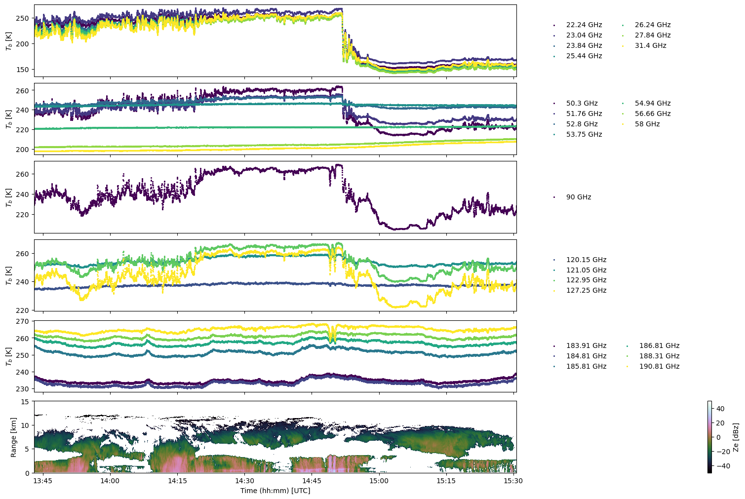
View data along a specific transect

Using the start and end times for each segment, we can look at data specifically in certain regions. For example at the southward leg “high level 9”.

# list all segments
for segment in flight['segments']:
    print(segment['name'])

major ascent
high level 1
long turn
high level 2
long turn
small ascent 1
high level 3
long turn
high level 4
long turn
high level 5
long turn
high level 6
long turn
high level 7
long turn
high level 8
long turn
high level 9
short turn
high level 10
major descent

flight_query = flightphase.FlightPhaseFile(flight)

attribute = 'name'
value = 'high level 9'

queried = flight_query.select(attribute, value) 
queried

[{'dropsondes': ['HALO-AC3_HALO_RF03_DS12',
   'HALO-AC3_HALO_RF03_DS13',
   'HALO-AC3_HALO_RF03_DS14',
   'HALO-AC3_HALO_RF03_DS15',
   'HALO-AC3_HALO_RF03_DS16'],
  'end': datetime.datetime(2022, 3, 13, 15, 30, 43),
  'irregularities': [],
  'kinds': ['high_level'],
  'levels': [40800],
  'name': 'high level 9',
  'segment_id': 'HALO-AC3_HALO_RF03_hl09',
  'start': datetime.datetime(2022, 3, 13, 13, 43, 1)}]

segment = queried[0]

t = dict(time=slice(segment['start'], segment['end']))

fig, (ax1, ax2, ax3, ax4, ax5, ax6) = plt.subplots(6, 1, sharex=True, gridspec_kw=dict(height_ratios=(1, 1, 1, 1, 1, 1)), constrained_layout=True, figsize=(15, 10))

kwargs = dict(s=5, linewidths=0)
colors = cm.get_cmap('viridis', 7).colors
for i in range(0, 7):
    ax1.scatter(ds_hamp_kv.time.sel(**t), ds_hamp_kv.TBs.sel(number_frequencies=i, **t), 
                label='%g GHz'%ds_hamp_kv.Freq[i], color=colors[i], **kwargs)

for i in range(7, 14):
    ax2.scatter(ds_hamp_kv.time.sel(**t), ds_hamp_kv.TBs.sel(number_frequencies=i, **t), 
                label='%g GHz'%ds_hamp_kv.Freq[i], color=colors[i-7], **kwargs)

ax1.legend(frameon=False, bbox_to_anchor=(1.05, 0.5), loc='center left', ncol=2)
ax2.legend(frameon=False, bbox_to_anchor=(1.05, 0.5), loc='center left', ncol=2)

ax1.set_ylabel('$T_b$ [K]')
ax2.set_ylabel('$T_b$ [K]')

colors = cm.get_cmap('viridis', 5).colors
for i in range(0, 1):
    ax3.scatter(ds_hamp_119.time.sel(**t), ds_hamp_119.TBs.sel(number_frequencies=i, **t), label='%g GHz'%ds_hamp_119.Freq[i], color=colors[i], **kwargs)

for i in range(1, 5):
    ax4.scatter(ds_hamp_119.time.sel(**t), ds_hamp_119.TBs.sel(number_frequencies=i, **t), label='%g GHz'%ds_hamp_119.Freq[i], color=colors[i-1], **kwargs)

ax3.legend(frameon=False, bbox_to_anchor=(1.05, 0.5), loc='center left')
ax4.legend(frameon=False, bbox_to_anchor=(1.05, 0.5), loc='center left')
    
ax3.set_ylabel('$T_b$ [K]')
ax4.set_ylabel('$T_b$ [K]')

colors = cm.get_cmap('viridis', 6).colors
for i in range(0, 6):
    ax5.scatter(ds_hamp_183.time.sel(**t), ds_hamp_183.TBs.sel(number_frequencies=i, **t), label='%g GHz'%ds_hamp_183.Freq[i], color=colors[i], **kwargs)

ax5.legend(frameon=False, bbox_to_anchor=(1.05, 0.5), loc='center left', ncol=2)

ax5.set_ylabel('$T_b$ [K]')

im = ax6.pcolormesh(ds_hamp_mira.time.sel(**t), ds_hamp_mira.range*1e-3, 10*np.log10(ds_hamp_mira.Ze.sel(**t).T), vmin=-50, vmax=50, cmap='cubehelix', shading='nearest')
ax6.set_xlim(segment['start'], segment['end'])
ax6.set_ylim([15, 0])
ax6.set_ylabel('Range [km]')
ax6.xaxis.set_major_formatter(mdates.DateFormatter('%H:%M'))
ax6.set_xlabel('Time (hh:mm) [UTC]')

fig.colorbar(im, ax=ax6, label='Ze [dBz]')

plt.show()