PMS probes and Nevzorov#

The following example presents the data collected by the PMS and Nevzorov probes on Polar 5 during the AFLUX and MOSAiC-ACA campaigns. The PMS probes where attached to the wings of the aircraft and operated by the group at DLR e.V. and JGU Mainz namely: C. Voigt, M. Moser, Yvonne Boose, and V. Hahn. If you have questions or if you would like to use the data for a publication, please get in contact with the dataset authors as stated above and in the dataset attributes contact or author. The data has been uploaded to the PANGAEA data base for both campaigns: AFLUX and MOSAiC-ACA.

Data access#

To analyse the data they first have to be loaded by importing the (AC)³ airborne meta data catalogue. To do so the ac3airborne package has to be installed. More information on how to do that and about the catalog can be found here.

import ac3airborne
cat = ac3airborne.get_intake_catalog()

Load Polar 5 flight phase information#

Polar 5 flights are divided into segments to easily access start and end times of flight patterns. For more information have a look at the respective github repository.

At first we want to load the flight segments of (AC)³airborne

meta = ac3airborne.get_flight_segments()
flight = meta['MOSAiC-ACA']['P5'][flight_id]

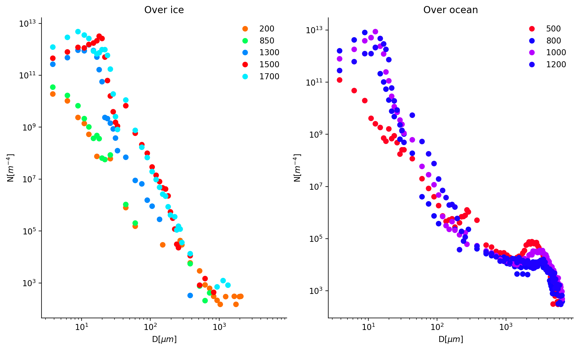
Here, we want to have a look on the size distributions measured during different legs of a racetrack_pattern. In order to simplify things we can import the module flightphase from the ac3airborne.tools.

from ac3airborne.tools import flightphase

We can now select only the racetrack_pattern. This kind of pattern is available two times.

flight_query = flightphase.FlightPhaseFile(flight)
queried = flight_query.selectKind(['racetrack_pattern'])
len(queried)

/home/mech/.local/lib/python3.10/site-packages/ac3airborne/tools/flightphase.py:27: UserWarning: the segment MOSAiC-ACA_P5_RF11_rt01 contains following irregularities: first leg begins far away from starting point of the other legs and is therefore longer
  warnings.warn(str)

Plots#

%matplotlib inline
import matplotlib.pyplot as plt
import matplotlib.dates as mdates
plt.style.use("../../mplstyle/book")

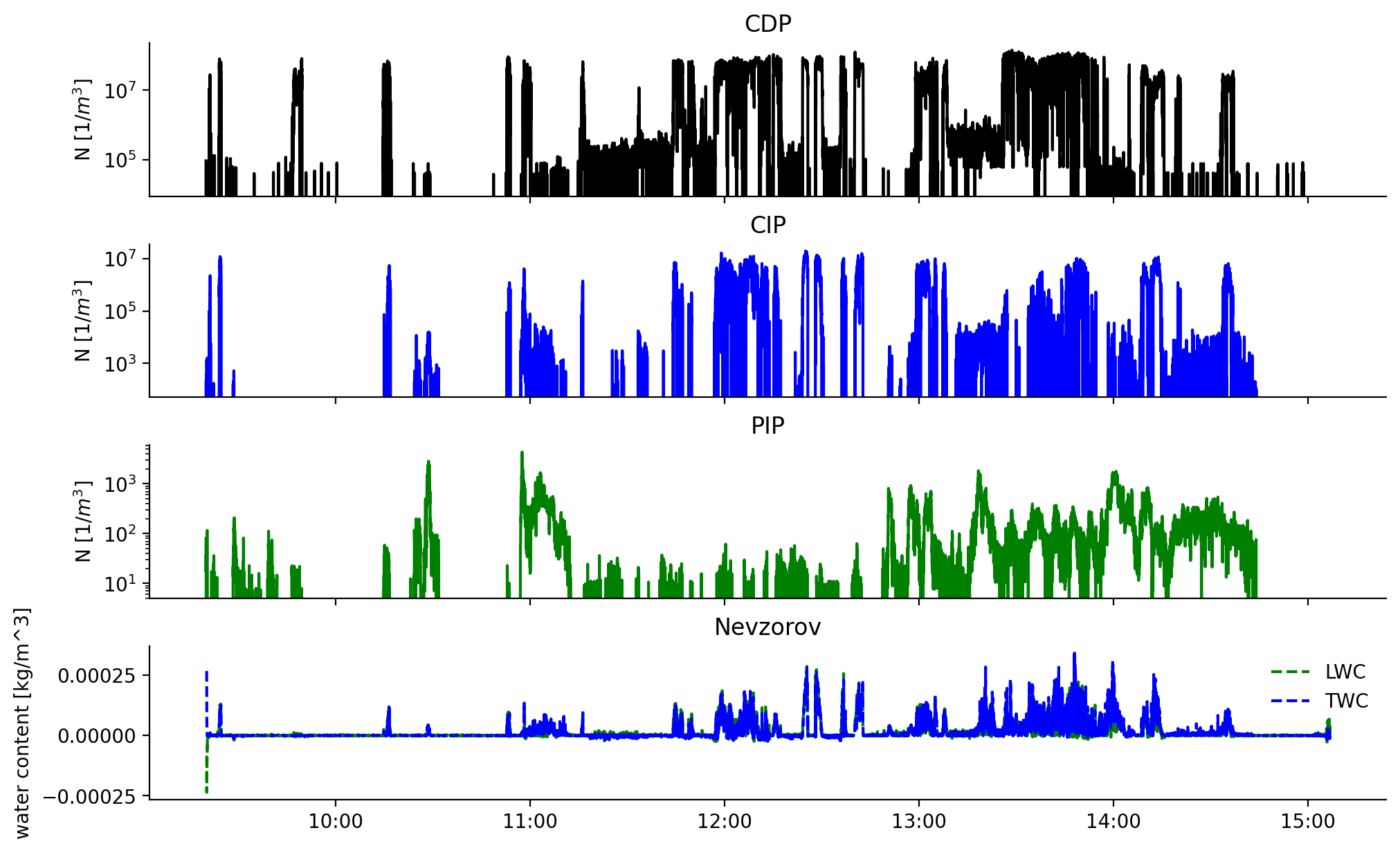
fig, (ax1, ax2, ax3, ax4) = plt.subplots(4, 1, sharex=True, gridspec_kw=dict(height_ratios=(1, 1, 1, 1)))
ax1.semilogy(ds_cdp.time, ds_cdp.N, color='k')
ax1.set_title('CDP')
ax2.semilogy(ds_cip.time, ds_cip.N, color='b')
ax2.set_title('CIP')
ax3.semilogy(ds_pip.time, ds_pip.N, color='g')
ax3.set_title('PIP')
ax4.plot(ds_nevzorov.time, ds_nevzorov.lwc, '--', color='g', label='LWC')
ax4.plot(ds_nevzorov.time, ds_nevzorov.twc, '--', color='b', label='TWC')
ax4.set_title('Nevzorov')

ax1.set_ylabel('N [$1/m^3$]')
ax2.set_ylabel('N [$1/m^3$]')
ax3.set_ylabel('N [$1/m^3$]')

ax4.set_ylabel('water content [kg/m^3]')

ax4.legend(frameon=False, loc='upper right')

ax4.xaxis.set_major_formatter(mdates.DateFormatter('%H:%M'))

plt.show()

from matplotlib import cm
import numpy as np
def colors(n):
    """Creates set of random colors of length n"""
    
    cmap = cm.get_cmap('gist_rainbow')
    rnd = np.random.uniform(low=0, high=1, size=n)
    cols = cmap(rnd)
    
    return cols

titles = ['ice','ocean']
fig, axs = plt.subplots(1, 2, gridspec_kw=dict())
for i, rtp in enumerate(queried):
    col_segments = colors(len(rtp['parts']))
    for j,part in enumerate(rtp['parts']):
        if 'leg' in part['name']:
            ds_sel = ds_pms_combined.sel(time=slice(part['start'],part['end']))
            axs[i].loglog(ds_sel.bin_mid, ds_sel.dNdD.mean(dim='time'), 'o',color=col_segments[j],label=part['levels'][0])
    axs[i].legend(frameon=False)
    axs[i].set_xlabel('D[$\mu m$]')
    axs[i].set_ylabel('N[$m^{-4}$]')
    axs[i].set_title('Over '+titles[i])

how_to_ac3airborne

PMS probes and Nevzorov

Contents

PMS probes and Nevzorov#

Data access#

Nevzorov#

PMS#

Load Polar 5 flight phase information#

Plots#