AMALi

AMALi#

During all campaigns, except HAMAG, the Airborne Mobile Aerosol Lidar for Arctic research (AMALi; Stachlewska et al., 2014) has been operated onboard the Polar 5. From the backscatter signal, a cloud mask and cloud top heights were derived. The dataset is available on the PANGAEA database for ACLOUD, AFLUX, MOSAiC-ACA, and HALO-AC3 and for COMPEX-EC and COMPEX on request.

If you have questions or if you would like to use the data for a publication, please don’t hesitate to get in contact with the dataset authors as stated in the dataset attributes contact or author.

import os

# local caching
try:
    from dotenv import load_dotenv

    load_dotenv()

    local_storage = os.environ['INTAKE_CACHE']
except ImportError:
    local_storage = '/tmp/'

kwds = {'simplecache': dict(
    cache_storage=local_storage, 
    same_names=True
)}

# needed for data stored in AC3 cloud
try:
    ac3cloud_username = os.environ['AC3_USER']
    ac3cloud_password = os.environ['AC3_PASSWORD']
    credentials = dict(user=ac3cloud_username, password=ac3cloud_password)
except ImportError:
    credentials = {}
    print("Only publicaly available datasets from ACLOUD, AFLUX, MOSAiC-ACA, and HALO-AC3 are accessible!")

First, we import the airborne catalogues to get the meta information of the datasets. To do so the ac3airborne package has to be installed. More information on how to do that and about the catalog can be found here.

import ac3airborne

cat = ac3airborne.get_intake_catalog()

datasets = []
for campaign in ['ACLOUD', 'AFLUX', 'MOSAiC-ACA','HALO-AC3','COMPEX-EC','COMPEX']:
    datasets.extend(list(cat[campaign]['P5']['AMALi']))
print(datasets)

['ACLOUD_P5_RF04', 'ACLOUD_P5_RF05', 'ACLOUD_P5_RF06', 'ACLOUD_P5_RF07', 'ACLOUD_P5_RF08', 'ACLOUD_P5_RF10', 'ACLOUD_P5_RF11', 'ACLOUD_P5_RF13', 'ACLOUD_P5_RF14', 'ACLOUD_P5_RF16', 'ACLOUD_P5_RF17', 'ACLOUD_P5_RF18', 'ACLOUD_P5_RF19', 'ACLOUD_P5_RF20', 'ACLOUD_P5_RF21', 'ACLOUD_P5_RF22', 'ACLOUD_P5_RF23', 'ACLOUD_P5_RF25', 'AFLUX_P5_RF03', 'AFLUX_P5_RF04', 'AFLUX_P5_RF05', 'AFLUX_P5_RF06', 'AFLUX_P5_RF07', 'AFLUX_P5_RF08', 'AFLUX_P5_RF09', 'AFLUX_P5_RF10', 'AFLUX_P5_RF11', 'AFLUX_P5_RF12', 'AFLUX_P5_RF13', 'AFLUX_P5_RF14', 'AFLUX_P5_RF15', 'MOSAiC-ACA_P5_RF04', 'MOSAiC-ACA_P5_RF05', 'MOSAiC-ACA_P5_RF06', 'MOSAiC-ACA_P5_RF07', 'MOSAiC-ACA_P5_RF08', 'MOSAiC-ACA_P5_RF09', 'MOSAiC-ACA_P5_RF10', 'MOSAiC-ACA_P5_RF11', 'HALO-AC3_P5_RF01', 'HALO-AC3_P5_RF03', 'HALO-AC3_P5_RF04', 'HALO-AC3_P5_RF05', 'HALO-AC3_P5_RF07', 'HALO-AC3_P5_RF08', 'HALO-AC3_P5_RF09', 'HALO-AC3_P5_RF10', 'HALO-AC3_P5_RF11', 'HALO-AC3_P5_RF12', 'HALO-AC3_P5_RF13', 'COMPEX-EC_P5_RF01', 'COMPEX-EC_P5_RF02', 'COMPEX-EC_P5_RF03', 'COMPEX-EC_P5_RF04', 'COMPEX-EC_P5_RF05', 'COMPEX-EC_P5_RF06', 'COMPEX-EC_P5_RF07', 'COMPEX_P5_RF01', 'COMPEX_P5_RF02', 'COMPEX_P5_RF03', 'COMPEX_P5_RF04', 'COMPEX_P5_RF05', 'COMPEX_P5_RF06', 'COMPEX_P5_RF07', 'COMPEX_P5_RF08', 'COMPEX_P5_RF09', 'COMPEX_P5_RF10', 'COMPEX_P5_RF11', 'COMPEX_P5_RF12', 'COMPEX_P5_RF13', 'COMPEX_P5_RF14', 'COMPEX_P5_RF15']

flight_id = 'COMPEX_P5_RF08'
campaign,platform,rf = flight_id.split('_')

We will load the level 1 dataset for a specific flight and see what can be found in there. ds_amali shows all relevant information on the dataset, such as author, contact, or citation information.

And the same for ds_cloud_top_height and ds_cloud_mask, the level 2 datasets with derived cloud top heights and the clodu mask based on AMALi.

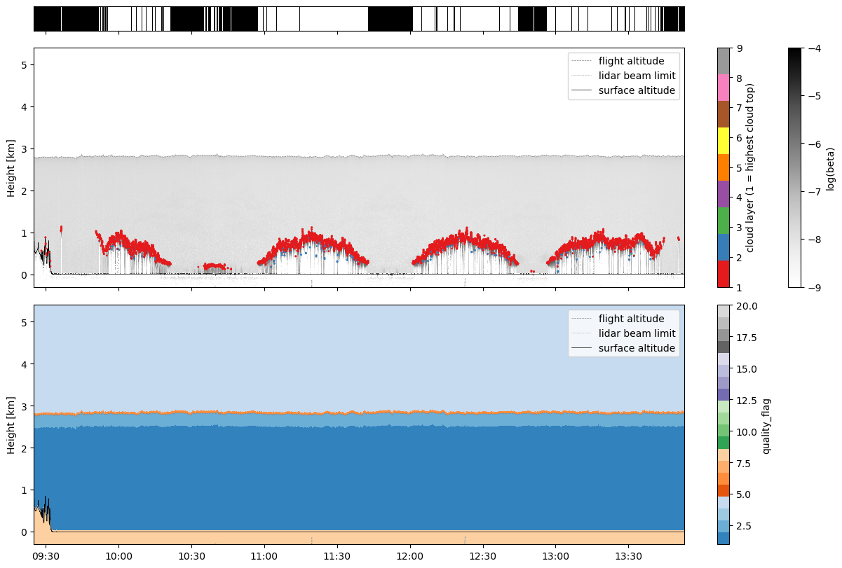
The datasets include attenuated backscatter signal for each channel (level 1 ds_amali: log_beta), the cloud top height (level 2 ds_cloud_top_height: cloud_top_height) and the number of cloud layers (level 2 ds_cloud_top_height: n_cloud_layer), and a cloud mask derived from the optical depth (level 2 ds_cloud_mask: cloud_mask). Additionally, the instrument status is provided and positional data of the aircraft (lat, lon, alt).

Load Polar 5 flight phase information#

Polar 5 flights are divided into segments to easily access start and end times of flight patterns. For more information have a look at the respective github repository.

At first we want to load the flight segments of (AC)³airborne

meta = ac3airborne.get_flight_segments() 

The following command lists all flight segments into the dictionary segments

segments = {s.get("segment_id"): {**s, "flight_id": flight["flight_id"]}
            for campaign in meta.values()
            for platform in campaign.values()
            for flight in platform.values()
            for s in flight["segments"]
            }

In this example we want to look at a high-level segment during COMPEX_P5_RF08, the EarthCARE collocation of RF08 during COMPEX.

seg = segments[flight_id+"_hl03"]

Using the start and end times of the segment stored in seg, we slice the MiRAC data to this flight section.

ds_cloud_top_height_sel = ds_cloud_top_height.sel(time=slice(seg["start"], seg["end"]))
ds_cloud_mask_sel = ds_cloud_mask.sel(time=slice(seg["start"], seg["end"]))

Plots#

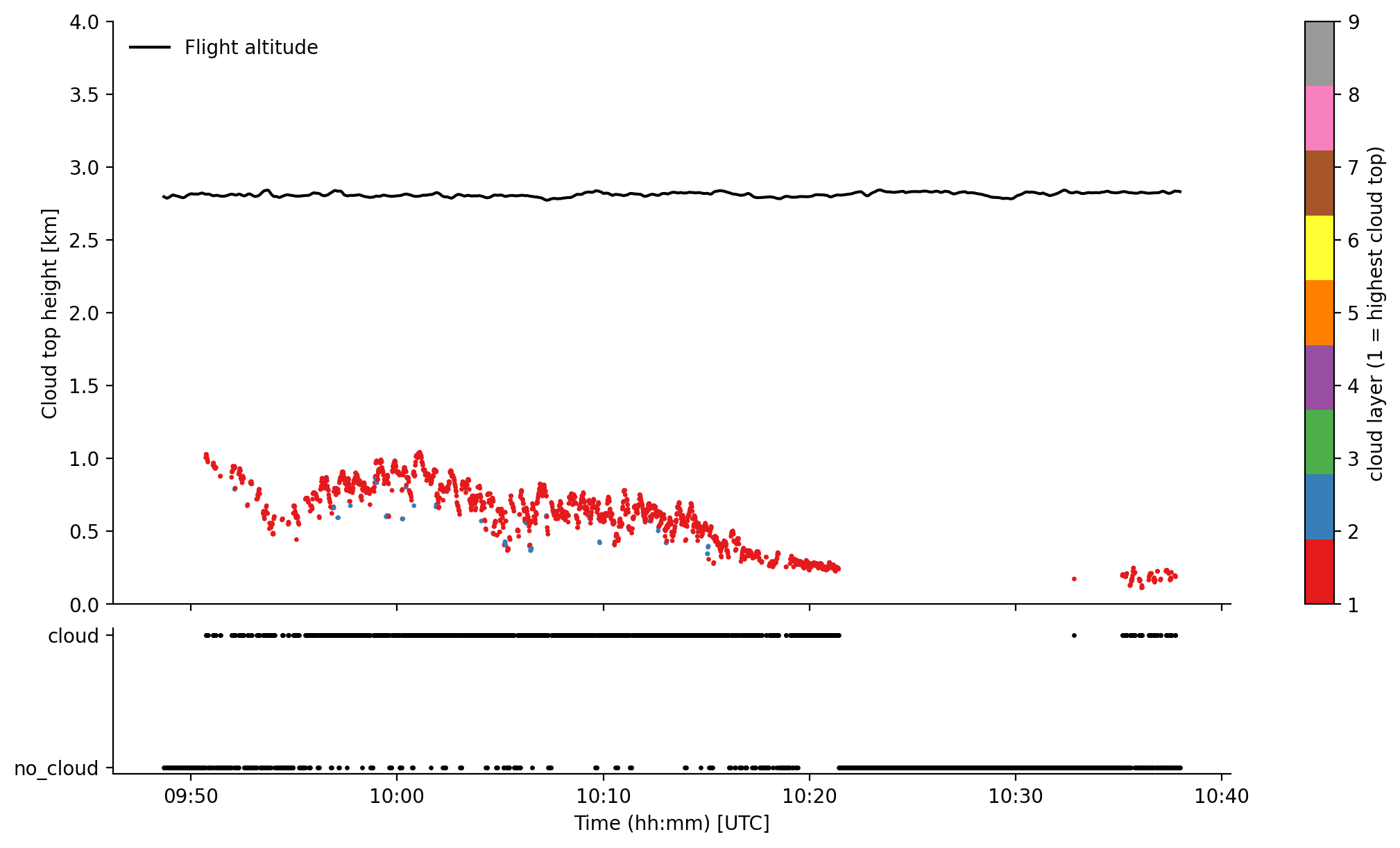
The flight section during ACLOUD RF05 is flown at about 3 km altitude in west-east direction during a cold-air outbreak event perpendicular to the wind field. Clearly one can identify the roll-cloud structure in the radar reflectivity and the 89 GHz brightness temperature.

%matplotlib inline
import matplotlib.pyplot as plt
import matplotlib.dates as mdates
plt.style.use("../../mplstyle/book")

fig, (ax1, ax2) = plt.subplots(2, 1, sharex=True, gridspec_kw=dict(height_ratios=[1, 0.25]))

# 1st: plot flight altitude and cloud top height with seperate colors for each layer
ax1.plot(ds_cloud_top_height_sel.time, ds_cloud_top_height_sel.alt*1e-3, color='k', label='Flight altitude')

stack = ds_cloud_top_height_sel.cth.stack({'tl': ['time', 'cloud_layer']})
im = ax1.scatter(x=stack.time, y=stack*1e-3, c=stack.cloud_layer, s=2, vmin=1, vmax=9, cmap='Set1')
fig.colorbar(im, ax=ax1, label='cloud layer (1 = highest cloud top)')
ax1.set_ylim(0, 4)
ax1.set_ylabel('Cloud top height [km]')

ax1.legend(frameon=False, loc='upper left')

# 3rd: plot cloud mask in lower part of the figure
ax2.scatter(ds_cloud_mask_sel.time, ds_cloud_mask_sel.cloud_mask, s=2, color='k')
ax2.set_yticks([int(x) for x in ds_cloud_mask_sel.cloud_mask.attrs['flag_values']])
ax2.set_yticklabels([x for x in ds_cloud_mask_sel.cloud_mask.attrs['flag_meanings'].split(' ')])
ax2.set_xlabel('Time (hh:mm) [UTC]')

ax2.xaxis.set_major_formatter(mdates.DateFormatter('%H:%M'))

plt.show()

../../_images/7239dcc2dbc7cf550debec3c8f95bc243436c759b9ba0a68303622a41ffb46fb.png

AMALi

Contents

AMALi#

Plot the data#

Load Polar 5 flight phase information#

Plots#