CMP22, CGR4 and KT-19#

The following example demonstrates the use of broadband irradiance data collected during ACLOUD and AFLUX. The dataset includes solar and terrestrial broadband irradiance and nadir brightness temperature. The full dataset is available on PANGAEA for ACLOUD and AFLUX.

Broadband irradiance (CMP22 pyranometer and CGR4 pyrgeometer)#

Upward and downward broadband irradiances are measured by pairs of CMP 22 pyranometers and CGR4 pyrgeometers, covering the solar (0.2–3.6 µm) and thermal-infrared (4.5–42 µm) wavelength range, respectively. Data is sampled with a frequency of 20 Hz. In stationary operation, the uncertainty of the sensors is less than 3 %.

Nadir brightness temperature (KT-19)#

Surface brightness temperature was measured by a nadir-looking Kelvin infrared radiation Thermometer (KT-19). These measurements were converted into surface temperature values assuming an emissivity of one. This is justified due to the small impact of atmospheric absorption in the wavelength range of 9.6 to 11.5 µm for which the KT-19 is sensitive. With a sampling frequency of 20 Hz, the KT-19 resolves small scales of the surface temperature heterogeneities, such as observed in the case of leads in sea ice.

More information about the dataset can be found in Ehrlich et al. 2019.

Data access#

To analyse the data they first have to be loaded by importing the (AC)³airborne meta data catalogue. To do so the ac3airborne package has to be installed. More information on how to do that and about the catalog can be found here.

Load Polar 5 flight phase information¶#

Polar 5 flights are divided into segments to easily access start and end times of flight patterns. For more information have a look at the respective github repository.

At first we want to load the flight segments of (AC)³airborne

meta = ac3airborne.get_flight_segments()

In this example we want to look at AFLUX_P5_RF03.

flight = meta['AFLUX']['P5']['AFLUX_P5_RF03']

We do not want to look into the data of the whole flight. Instead we want to select a specific portion of the flight, for example a high_level leg. In order to simplify things we can import the module flightphase from the ac3airborne.tools.

from ac3airborne.tools import flightphase as fp

We can now select only the high_level legs and show a list of the available legs of this kind.

flight_query = fp.FlightPhaseFile(flight)
queried = flight_query.selectKind(['high_level'])
queried

[{'dropsondes': [],
  'end': datetime.datetime(2019, 3, 21, 10, 44, 51),
  'irregularities': [],
  'kinds': ['high_level'],
  'levels': [9500],
  'name': 'high level 1',
  'segment_id': 'AFLUX_P5_RF03_hl01',
  'start': datetime.datetime(2019, 3, 21, 10, 5, 48)},
 {'dropsondes': [],
  'end': datetime.datetime(2019, 3, 21, 12, 53, 41),
  'irregularities': [],
  'kinds': ['high_level'],
  'levels': [9500],
  'name': 'high level 2',
  'segment_id': 'AFLUX_P5_RF03_hl02',
  'start': datetime.datetime(2019, 3, 21, 12, 44, 57)},
 {'dropsondes': [],
  'end': datetime.datetime(2019, 3, 21, 14, 6, 37),
  'irregularities': [],
  'kinds': ['high_level'],
  'levels': [9500],
  'name': 'high level 3',
  'segment_id': 'AFLUX_P5_RF03_hl03',
  'start': datetime.datetime(2019, 3, 21, 13, 35, 32)}]

We decide to select a specific element of the array:

queried[1]

{'dropsondes': [],
 'end': datetime.datetime(2019, 3, 21, 12, 53, 41),
 'irregularities': [],
 'kinds': ['high_level'],
 'levels': [9500],
 'name': 'high level 2',
 'segment_id': 'AFLUX_P5_RF03_hl02',
 'start': datetime.datetime(2019, 3, 21, 12, 44, 57)}

We will use the start and end time later in order to select the data for the analysis.

start = queried[1]['start']
end   = queried[1]['end']

Plots#

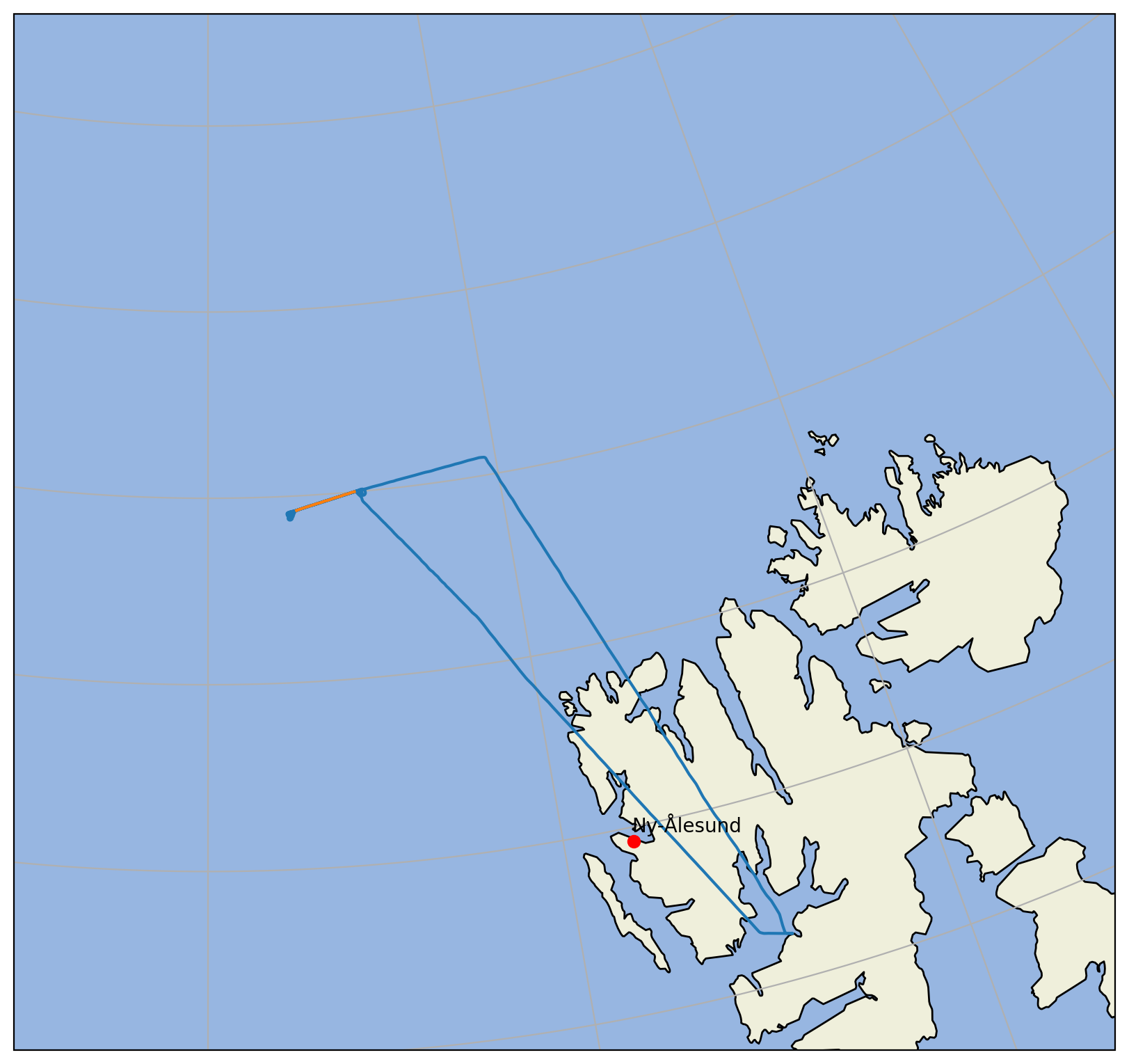
Plot the fligt segment#

Now we can plot both the whole flight and the flight segment, so that we can show where the measurments have taken place before we plot them.

import matplotlib.pyplot as plt
import cartopy.crs as ccrs
import cartopy.feature as cfeature
plt.style.use("../../mplstyle/book")

proj = ccrs.NorthPolarStereo()
extent = (-5.0, 24.0, 78.0, 83.0)

fig = plt.figure(figsize=(8, 8))
ax = plt.axes(projection=proj)
ax.set_extent(extent)

ax.add_feature(cfeature.OCEAN)
ax.add_feature(cfeature.LAND)
ax.gridlines()
ax.coastlines()

nya_lat = 78.924444
nya_lon = 11.928611

ax.plot(nya_lon, nya_lat, 'ro', transform=ccrs.PlateCarree())
ax.text(nya_lon, nya_lat+0.05, 'Ny-Ålesund', transform=ccrs.PlateCarree())

line_all = ax.plot(ds_gps.lon, ds_gps.lat, transform=ccrs.PlateCarree())

line = ax.plot(ds_gps.lon.sel(time=slice(start, end)),
               ds_gps.lat.sel(time=slice(start, end)),
               transform=ccrs.PlateCarree())

plt.show()

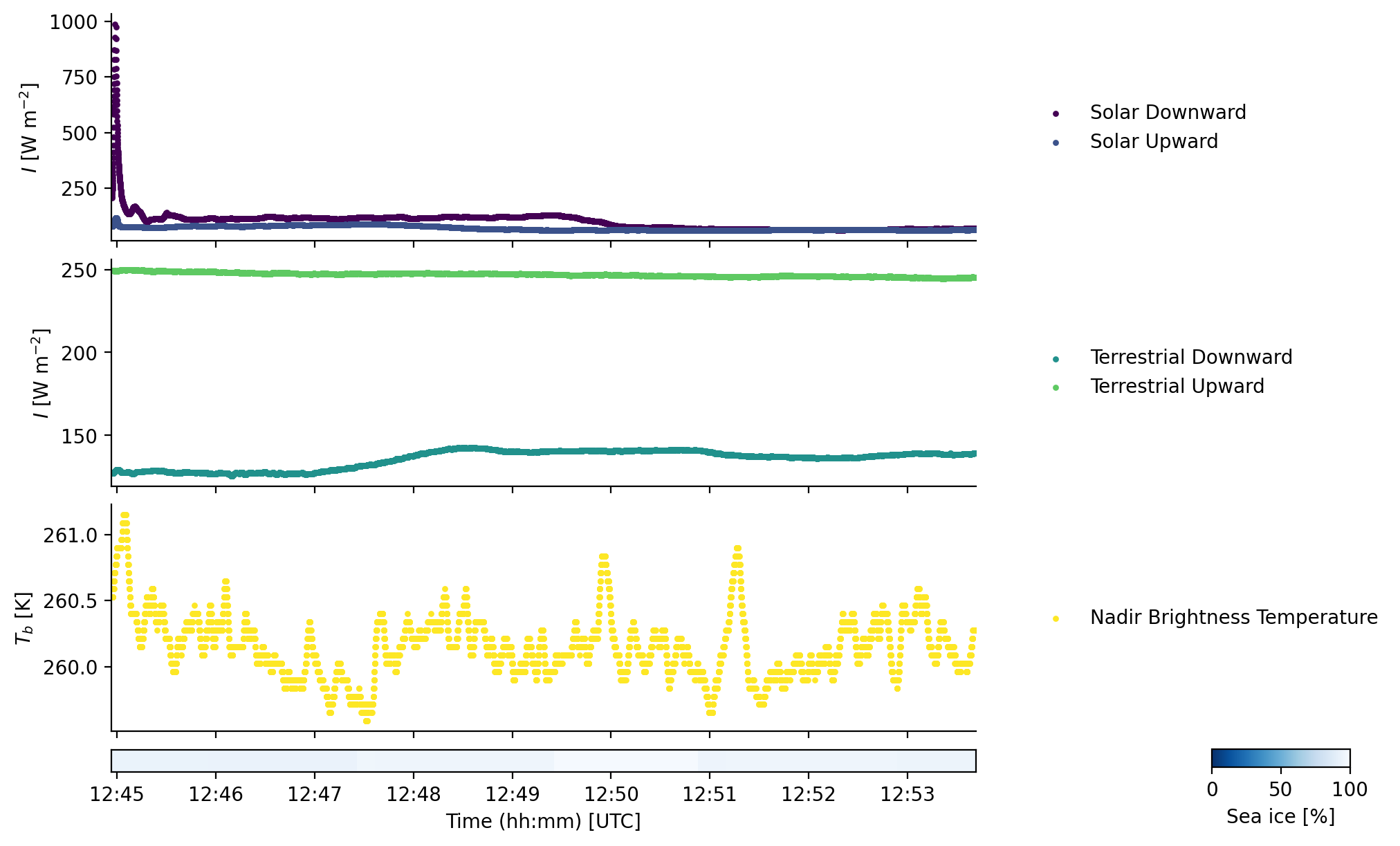
Plot the data#

We can now select the data and plot it.

time_of_segment = ds_broad_irr.time.sel(Time = slice(start, end))

Solar_F_dw = ds_broad_irr.Solar_F_dw.sel(Time = slice(start, end))
Solar_F_up = ds_broad_irr.Solar_F_up.sel(Time = slice(start, end))
Terr_F_dw  = ds_broad_irr.Terr_F_dw.sel(Time = slice(start, end))
Terr_F_up  = ds_broad_irr.Terr_F_up.sel(Time = slice(start, end))
KT19       = ds_broad_irr.KT19.sel(Time = slice(start, end))

We want to add also some information about ice coverage:

ds_sea_ice = cat['AFLUX']['P5']['AMSR2_SIC']['AFLUX_P5_RF03'].to_dask().sel(time = slice(start, end))

import matplotlib.dates as mdates
from matplotlib import cm
import numpy as np
import warnings
warnings.filterwarnings("ignore")

fig, (ax1, ax2, ax3, ax4) = plt.subplots(4, 1, sharex=True, gridspec_kw=dict(height_ratios=(1, 1, 1, 0.1)))

kwargs = dict(s=10, linewidths=0)
colors = cm.get_cmap('viridis', 5).colors

ax1.scatter(time_of_segment, Solar_F_dw, label='Solar Downward', color=colors[0], **kwargs)
ax1.scatter(time_of_segment, Solar_F_up, label='Solar Upward', color=colors[1], **kwargs)

ax2.scatter(time_of_segment, Terr_F_dw, label='Terrestrial Downward', color=colors[2], **kwargs)
ax2.scatter(time_of_segment, Terr_F_up, label='Terrestrial Upward', color=colors[3], **kwargs)

ax3.scatter(time_of_segment, KT19, label='Nadir Brightness Temperature', color=colors[4], **kwargs)

ax1.legend(frameon=False, bbox_to_anchor=(1.05, 0.5), loc='center left')
ax2.legend(frameon=False, bbox_to_anchor=(1.05, 0.5), loc='center left')
ax3.legend(frameon=False, bbox_to_anchor=(1.05, 0.5), loc='center left')

ax1.set_ylabel('$I$ [W m$^{-2}$]')
ax2.set_ylabel('$I$ [W m$^{-2}$]')
ax3.set_ylabel('$T_b$ [K]')

# plot AMSR2 sea ice concentration
im = ax4.pcolormesh(ds_sea_ice.time,
               np.array([0, 1]),
               np.array([ds_sea_ice.sic,ds_sea_ice.sic]), cmap='Blues_r', vmin=0, vmax=100,
               shading='auto')
cax = fig.add_axes([0.87, 0.085, 0.1, ax4.get_position().height])
fig.colorbar(im, cax=cax, orientation='horizontal', label='Sea ice [%]')
ax4.tick_params(axis='y', labelleft=False, left=False)
ax4.spines[:].set_visible(True)

ax4.xaxis.set_major_formatter(mdates.DateFormatter('%H:%M'))
ax4.set_xlabel('Time (hh:mm) [UTC]')

plt.show()

how_to_ac3airborne

CMP22, CGR4 and KT-19

Contents

CMP22, CGR4 and KT-19#

Broadband irradiance (CMP22 pyranometer and CGR4 pyrgeometer)#

Nadir brightness temperature (KT-19)#

Data access#

Get data#

Load Polar 5 flight phase information¶#

Read the GPS information#

Plots#

Plot the fligt segment#

Plot the data#