HATPRO#
The following example presents the nadir passive microwave radiometer HATPRO. The Humidity And Temperature PROfiler (HATPRO) replaced the MiRAC-P radiometer during the MOSAiC-ACA campaign.
If you have questions or if you would like to use the data for a publication, please don’t hesitate to get in contact with the dataset authors as stated in the dataset attributes contact or author.
import os
from dotenv import load_dotenv

load_dotenv()

# local caching
kwds = {'simplecache': dict(
    cache_storage=os.environ['INTAKE_CACHE'],
    same_names=True
)}
To analyse the data they first have to be loaded by importing the (AC)3 airborne meta data catalogue. To do so the ac3airborne package has to be installed. More information on how to do that and about the catalog can be found here.
import ac3airborne
cat = ac3airborne.get_intake_catalog()

datasets = []
for campaign in ['MOSAiC-ACA','HALO-AC3']:
    datasets.extend(list(cat[campaign]['P5']['HATPRO']))
datasets
['MOSAiC-ACA_P5_RF02',
 'MOSAiC-ACA_P5_RF04',
 'MOSAiC-ACA_P5_RF05',
 'MOSAiC-ACA_P5_RF06',
 'MOSAiC-ACA_P5_RF07',
 'MOSAiC-ACA_P5_RF08',
 'MOSAiC-ACA_P5_RF09',
 'MOSAiC-ACA_P5_RF10',
 'MOSAiC-ACA_P5_RF11',
 'HALO-AC3_P5_RF01',
 'HALO-AC3_P5_RF02',
 'HALO-AC3_P5_RF03',
 'HALO-AC3_P5_RF04',
 'HALO-AC3_P5_RF05',
 'HALO-AC3_P5_RF06',
 'HALO-AC3_P5_RF07',
 'HALO-AC3_P5_RF08',
 'HALO-AC3_P5_RF09',
 'HALO-AC3_P5_RF10',
 'HALO-AC3_P5_RF11',
 'HALO-AC3_P5_RF12',
 'HALO-AC3_P5_RF13']
Note
Have a look at the attributes of the xarray dataset ds_hatpro for all relevant information on the dataset, such as author, contact, or citation information.
ds_hatpro = cat['MOSAiC-ACA']['P5']['HATPRO']['MOSAiC-ACA_P5_RF11'](storage_options=kwds).to_dask()
ds_hatpro
/net/sever/mech/miniconda3/envs/howtoac3/lib/python3.11/site-packages/intake_xarray/base.py:21: FutureWarning: The return type of `Dataset.dims` will be changed to return a set of dimension names in future, in order to be more consistent with `DataArray.dims`. To access a mapping from dimension names to lengths, please use `Dataset.sizes`.
  'dims': dict(self._ds.dims),
<xarray.Dataset> Size: 1MB
Dimensions:    (channel: 14, time: 15553)
Coordinates:
  * time       (time) datetime64[ns] 124kB 2020-09-13T09:20:01 ... 2020-09-13...
  * channel    (channel) int64 112B 0 1 2 3 4 5 6 7 8 9 10 11 12 13
Data variables:
    frequency  (channel) float32 56B ...
    tb         (time, channel) float32 871kB ...
    lon        (time) float64 124kB ...
    lat        (time) float64 124kB ...
Attributes: (12/14)
    institution:  Institute for Geophysics and Meteorology (IGM), University ...
    source:       airborne observation
    references:   https://doi.org/10.1016/j.atmosres.2004.12.005
    author:       Nils Risse
    convention:   CF-1.8
    featureType:  trajectory
    ...           ...
    flight_id:    RF11
    title:        HATPRO brightness temperature
    instrument:   HATPRO: Humidity and Temperature Profiler
    history:      measured onboard Polar 5 during MOSAiC-ACA campaign; proces...
    contact:      mario.mech@uni-koeln.de, n.risse@uni-koeln.de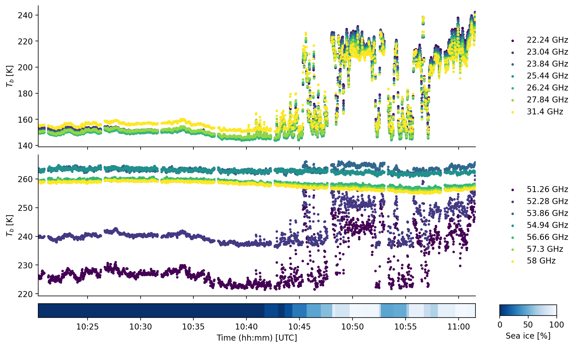
created: 2021-11-09The dataset includes brightness temperatures (tb) observed by HATPRO at the 22 GHz water vapor absorption line (22.24, 23.04, 23.84, 25.44, 26.24, 27.84 GHz), at the 31.3 GHz window frequency and the 56 GHz oxygen absorption line (51.26, 52.28, 53.86, 54.94, 56.66, 57.3, 58.0 GHz).
Load Polar 5 flight phase information#
Polar 5 flights are divided into segments to easily access start and end times of flight patterns. For more information have a look at the respective github repository.
At first we want to load the flight segments of (AC)³airborne
meta = ac3airborne.get_flight_segments()
The following command lists all flight segments into the dictionary segments
segments = {s.get("segment_id"): {**s, "flight_id": flight["flight_id"]}
             for campaign in meta.values()
             for platform in campaign.values()
             for flight in platform.values()
             for s in flight["segments"]
            }
In this example we want to look at a high-level segment during MOSAiC-ACA RF11
seg = segments["MOSAiC-ACA_P5_RF11_hl05"]
Using the start and end times of the segment MOSAiC-ACA_P5_RF11_hl05 stored in seg, we slice the HATPRO data to the selected flight section.
ds_hatpro_sel = ds_hatpro.sel(time=slice(seg["start"], seg["end"]))
In polar regions, the surface type is helpful for the interpretation of airborne passive microwave observations, especially near the marginal sea ice zone, as generally a higher emissivity is expected over sea ice compared to open ocean. Therefore, we also load AMSR2 sea ice concentration data along the Polar 5 flight track, which is operationally derived by the University of Bremen.
ds_sea_ice = cat['MOSAiC-ACA']['P5']['AMSR2_SIC']['MOSAiC-ACA_P5_RF11'].to_dask().sel(
    time=slice(seg["start"], seg["end"]))
/net/sever/mech/miniconda3/envs/howtoac3/lib/python3.11/site-packages/intake_xarray/base.py:21: FutureWarning: The return type of `Dataset.dims` will be changed to return a set of dimension names in future, in order to be more consistent with `DataArray.dims`. To access a mapping from dimension names to lengths, please use `Dataset.sizes`.
  'dims': dict(self._ds.dims),
Plots#
import warnings
warnings.filterwarnings("ignore")
import matplotlib.pyplot as plt
import matplotlib.dates as mdates
from matplotlib import cm
import numpy as np
%matplotlib inline
plt.style.use("../../mplstyle/book")
fig, (ax1, ax2, ax3) = plt.subplots(3, 1, sharex=True, gridspec_kw=dict(height_ratios=(1, 1, 0.1)))

kwargs = dict(s=10, linewidths=0)
colors = cm.get_cmap('viridis', 7).colors
for i in range(0, 7):
    ax1.scatter(ds_hatpro_sel.time, ds_hatpro_sel.tb.sel(channel=i), label='%g GHz'%ds_hatpro_sel.frequency.sel(channel=i).item(), color=colors[i], **kwargs)

for i in range(7, 14):
    ax2.scatter(ds_hatpro_sel.time, ds_hatpro_sel.tb.sel(channel=i), label='%g GHz'%ds_hatpro_sel.frequency.sel(channel=i).item(), color=colors[i-7], **kwargs)

ax1.legend(frameon=False, bbox_to_anchor=(1.05, 0.5), loc='center left')
ax2.legend(frameon=False, bbox_to_anchor=(1.05, 0.5), loc='center left')

ax1.set_ylabel('$T_b$ [K]')
ax2.set_ylabel('$T_b$ [K]')

# plot AMSR2 sea ice concentration
im = ax3.pcolormesh(ds_sea_ice.time,
               np.array([0, 1]),
               np.array([ds_sea_ice.sic,ds_sea_ice.sic]), cmap='Blues_r', vmin=0, vmax=100,
               shading='auto')
cax = fig.add_axes([0.87, 0.085, 0.1, ax3.get_position().height])
fig.colorbar(im, cax=cax, orientation='horizontal', label='Sea ice [%]')
ax3.tick_params(axis='y', labelleft=False, left=False)
#ax4.spines[:].set_visible(True)
ax3.spines['top'].set_visible(True)
ax3.spines['right'].set_visible(True)

ax3.xaxis.set_major_formatter(mdates.DateFormatter('%H:%M'))
ax3.set_xlabel('Time (hh:mm) [UTC]')

plt.show()