MiRAC-A

The following example demonstrates the use of MiRAC-A data collected during ACLOUD, AFLUX, and MOSAiC-ACA. The Microwave Radar/Radiometer for Arctic Clouds (MiRAC) consists of an active component, a 94 GHz Frequency Modulated Continuous Wave (FMCW) cloud radar, and a passive 89 GHz microwave radiometer. MiRAC-A is mounted on Polar 5 with a fixed viewing angle of 25° against flight direction.

More information on the instrument can be found in Mech et al. (2019).

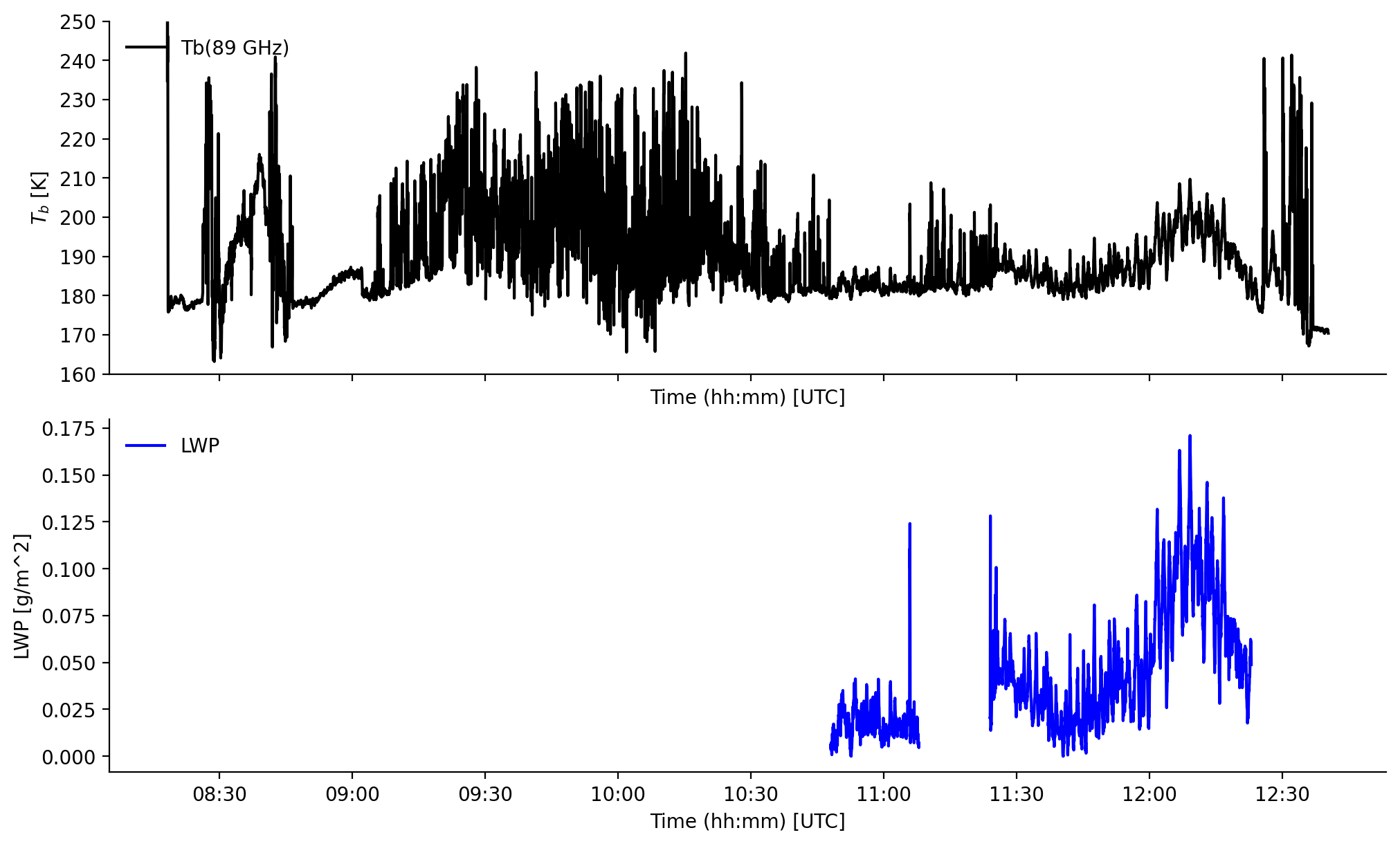
In addition, the liquid water path product over open ocean derived from the passive channel during the ACLOUD campaign Kliesch et al. (2021) is included.

If you have questions or if you would like to use the data for a publication, please don’t hesitate to get in contact with the dataset authors as stated in the dataset attributes contact or author.

Data access

Some of the data, like the preliminary data of the HALO-(AC)3 campaign, is stored on the (AC)3 nextcloud server. This requires username and password as credentials (registration) that need to be loaded from environment variables

import os
ac3cloud_username = os.environ['AC3_USER']
ac3cloud_password = os.environ['AC3_PASSWORD']

To analyse the data they first have to be loaded by importing the (AC)³ airborne meta data catalogue. To do so the ac3airborne package has to be installed. More information on how to do that and about the catalog can be found here.

import ac3airborne

cat = ac3airborne.get_intake_catalog()

datasets = []
for campaign in ['ACLOUD', 'AFLUX', 'MOSAiC-ACA','HALO-AC3']:
    datasets.extend(list(cat[campaign]['P5']['MiRAC-A']))
datasets

['ACLOUD_P5_RF04',
 'ACLOUD_P5_RF05',
 'ACLOUD_P5_RF06',
 'ACLOUD_P5_RF07',
 'ACLOUD_P5_RF08',
 'ACLOUD_P5_RF10',
 'ACLOUD_P5_RF11',
 'ACLOUD_P5_RF14',
 'ACLOUD_P5_RF15',
 'ACLOUD_P5_RF16',
 'ACLOUD_P5_RF17',
 'ACLOUD_P5_RF18',
 'ACLOUD_P5_RF19',
 'ACLOUD_P5_RF20',
 'ACLOUD_P5_RF21',
 'ACLOUD_P5_RF22',
 'ACLOUD_P5_RF23',
 'ACLOUD_P5_RF25',
 'AFLUX_P5_RF03',
 'AFLUX_P5_RF04',
 'AFLUX_P5_RF05',
 'AFLUX_P5_RF06',
 'AFLUX_P5_RF07',
 'AFLUX_P5_RF08',
 'AFLUX_P5_RF09',
 'AFLUX_P5_RF10',
 'AFLUX_P5_RF11',
 'AFLUX_P5_RF12',
 'AFLUX_P5_RF13',
 'AFLUX_P5_RF14',
 'AFLUX_P5_RF15',
 'MOSAiC-ACA_P5_RF05',
 'MOSAiC-ACA_P5_RF06',
 'MOSAiC-ACA_P5_RF07',
 'MOSAiC-ACA_P5_RF08',
 'MOSAiC-ACA_P5_RF09',
 'MOSAiC-ACA_P5_RF10',
 'MOSAiC-ACA_P5_RF11',
 'HALO-AC3_P5_RF01',
 'HALO-AC3_P5_RF03',
 'HALO-AC3_P5_RF04',
 'HALO-AC3_P5_RF05',
 'HALO-AC3_P5_RF07',
 'HALO-AC3_P5_RF08',
 'HALO-AC3_P5_RF09',
 'HALO-AC3_P5_RF10',
 'HALO-AC3_P5_RF11',
 'HALO-AC3_P5_RF12',
 'HALO-AC3_P5_RF13']

From here on, we work on a specific flight from the ACLOUD campaign ACLOUD_P5_RF05.

flight = 'ACLOUD_P5_RF05'
campaign, platform, rf = flight.split('_')

Note

Have a look at the attributes of the xarray dataset ds_mirac_a for all relevant information on the dataset, such as author, contact, or citation information.

ds_mirac_a = cat[campaign][platform]['MiRAC-A'][flight].to_dask()
ds_mirac_a

<xarray.Dataset>
Dimensions:        (time: 11765, height: 1400)
Coordinates:
  * time           (time) datetime64[ns] 2017-05-25T08:18:18 ... 2017-05-25T1...
  * height         (height) float32 -1e+03 -995.0 -990.0 ... 5.99e+03 5.995e+03
Data variables:
    Ze_unfiltered  (time, height) float32 ...
    Ze             (time, height) float32 ...
    tb             (time) float32 234.8 278.3 262.1 239.6 ... 170.7 170.5 170.4
    Ze_flag        (time, height) uint8 ...
    lon            (time) float32 15.42 15.41 15.41 15.41 ... 15.05 15.05 15.05
    lat            (time) float32 78.25 78.25 78.25 78.25 ... 78.29 78.29 78.29
    alt            (time) float32 147.6 156.0 163.8 178.6 ... 856.7 852.3 847.8
Attributes: (12/15)
    title:        MiRAC-A observations onboard Polar 5 during ACLOUD
    institution:  Institute for Geophysics and Meteorology (IGM), University ...
    source:       airborne observation
    history:      measured onboard Polar 5 during ACLOUD campaign; processed,...
    references:   https://doi.org/10.5194/amt-12-5019-2019
    comment:      the radar system and the 89 GHz channel were inclined by 25...
    ...           ...
    platform:     Polar 5
    flight_id:    RF05
    instrument:   MiRAC-A: Microwave Radar/radiometer for Arctic Clouds (active)
    author:       Nils Risse
    contact:      mario.mech@uni-koeln.de, n.risse@uni-koeln.de
    created:      2022-07-19

xarray.Dataset

• Dimensions:
  • time: 11765
  • height: 1400
• Coordinates: (2)
  • time
    (time)
    datetime64[ns]
    2017-05-25T08:18:18 ... 2017-05-...

    standard_name :

    time

    long_name :

    time in seconds since epoch

    array(['2017-05-25T08:18:18.000000000', '2017-05-25T08:18:19.000000000',
           '2017-05-25T08:18:20.000000000', ..., '2017-05-25T12:40:20.000000000',
           '2017-05-25T12:40:21.000000000', '2017-05-25T12:40:22.000000000'],
          dtype='datetime64[ns]')

  • height
    (height)
    float32
    -1e+03 -995.0 ... 5.995e+03

    standard_name :

    height

    long_name :

    radar bin height

    units :

    m

    comment :

    height of radar bins at lower boundary with resolution of 5 m

    array([-1000.,  -995.,  -990., ...,  5985.,  5990.,  5995.], dtype=float32)

• Data variables: (7)
  • Ze_unfiltered
    (time, height)
    float32
    ...

    standard_name :

    equivalent_reflectivity_factor

    long_name :

    equivalent radar reflectivity factor

    units :

    mm^6/m^3

    comment :

    original measurements corrected by +3 dB according to radar-manufacturer note (RPG-Radiometer Physics GmbH, 2018-08-30), unfiltered radar reflectivity interpolated to regular height grid and transformed to quasi-nadir observations

    [16471000 values with dtype=float32]

  • Ze
    (time, height)
    float32
    ...

    standard_name :

    equivalent_reflectivity_factor

    long_name :

    equivalent radar reflectivity factor

    units :

    mm^6/m^3

    comment :

    original measurements corrected by +3 dB according to radar-manufacturer note (RPG-Radiometer Physics GmbH, 2018-08-30), radar reflectivity interpolated to regular height grid, transformed to quasi-nadir observations, and filtered for disturbances (see Ze_flag)

    [16471000 values with dtype=float32]

  • tb
    (time)
    float32
    ...

    standard_name :

    brightness_temperature

    long_name :

    brightness temperature

    units :

    K

    description :

    89 GHz brightness temperature along slanted path

    comment :

    During low-level flights over surfaces with a high backscattering coefficient such as sea ice, the 89 GHz channel might be affected by noise transmitted by the cloud radar.

    array([234.79802, 278.25922, 262.102  , ..., 170.66077, 170.50888, 170.42293],
          dtype=float32)

  • Ze_flag
    (time, height)
    uint8
    ...

    standard_name :

    Ze_flag

    long_name :

    flag for equivalent radar reflectivity factor

    flag_masks :

    1 2 4 8

    flag_meanings :

    defective_gate_filter snr_filter speckle_filter subsurface_reflection_filter

    description :

    mask for filtered radar reflectivity bins during processing

    [16471000 values with dtype=uint8]

  • lon
    (time)
    float32
    ...

    standard_name :

    longitude

    long_name :

    WGS84 datum/longitude

    units :

    degrees_east

    array([15.416325, 15.41407 , 15.411834, ..., 15.046618, 15.049418, 15.052221],
          dtype=float32)

  • lat
    (time)
    float32
    ...

    standard_name :

    latitude

    long_name :

    WGS84 datum/latitude

    units :

    degrees_north

    array([78.24913 , 78.24927 , 78.24941 , ..., 78.29419 , 78.29407 , 78.293945],
          dtype=float32)

  • alt
    (time)
    float32
    ...

    standard_name :

    altitude

    long_name :

    aircraft flight altitude above mean sea level

    units :

    m

    array([147.64835, 156.0091 , 163.81396, ..., 856.6574 , 852.2666 , 847.8256 ],
          dtype=float32)

• Attributes: (15)

  title :

  MiRAC-A observations onboard Polar 5 during ACLOUD

  institution :

  Institute for Geophysics and Meteorology (IGM), University of Cologne

  source :

  airborne observation

  history :

  measured onboard Polar 5 during ACLOUD campaign; processed, quality-checked, and reformatted by University of Cologne

  references :

  https://doi.org/10.5194/amt-12-5019-2019

  comment :

  the radar system and the 89 GHz channel were inclined by 25 degrees. However, only Ze is already transformed to nadir.

  convention :

  CF-1.8

  featureType :

  trajectory

  mission :

  ACLOUD

  platform :

  Polar 5

  flight_id :

  RF05

  instrument :

  MiRAC-A: Microwave Radar/radiometer for Arctic Clouds (active)

  author :

  Nils Risse

  contact :

  mario.mech@uni-koeln.de, n.risse@uni-koeln.de

  created :

  2022-07-19

The dataset includes the radar reflectivity (Ze, Ze_unfiltered), the radar reflectivity filter mask (Ze_flag), the 89 GHz brightness temperature (TB_89) as well as information on the aircraft’s flight altitude (altitude). The radar reflectivity is defined on a regular time-height grid with corresponding target positions (lat, lon). The full dataset is available on PANGAEA.

Load Polar 5 flight phase information

Polar 5 flights are divided into segments to easily access start and end times of flight patterns. For more information have a look at the respective github repository.

At first we want to load the flight segments of (AC)³airborne

meta = ac3airborne.get_flight_segments()

The following command lists all flight segments into the dictionary segments

segments = {s.get("segment_id"): {**s, "flight_id": flight["flight_id"]}
             for campaign in meta.values()
             for platform in campaign.values()
             for flight in platform.values()
             for s in flight["segments"]
            }

In this example we want to look at a high-level segment during ACLOUD RF05

seg = segments[flight + "_hl09"]

Using the start and end times of the segment ACLOUD_P5_RF05_hl09 stored in seg, we slice the MiRAC data to this flight section.

ds_mirac_a_sel = ds_mirac_a.sel(time=slice(seg["start"], seg["end"]))

ds_mirac_a_sel

<xarray.Dataset>
Dimensions:        (time: 981, height: 1400)
Coordinates:
  * time           (time) datetime64[ns] 2017-05-25T11:28:15 ... 2017-05-25T1...
  * height         (height) float32 -1e+03 -995.0 -990.0 ... 5.99e+03 5.995e+03
Data variables:
    Ze_unfiltered  (time, height) float32 ...
    Ze             (time, height) float32 ...
    tb             (time) float32 187.6 188.3 188.1 187.5 ... 187.1 186.7 186.8
    Ze_flag        (time, height) uint8 ...
    lon            (time) float32 0.2009 0.2084 0.2121 ... 4.932 4.94 4.943
    lat            (time) float32 77.84 77.84 77.84 77.84 ... 77.83 77.83 77.83
    alt            (time) float32 2.9e+03 2.897e+03 ... 2.881e+03 2.882e+03
Attributes: (12/15)
    title:        MiRAC-A observations onboard Polar 5 during ACLOUD
    institution:  Institute for Geophysics and Meteorology (IGM), University ...
    source:       airborne observation
    history:      measured onboard Polar 5 during ACLOUD campaign; processed,...
    references:   https://doi.org/10.5194/amt-12-5019-2019
    comment:      the radar system and the 89 GHz channel were inclined by 25...
    ...           ...
    platform:     Polar 5
    flight_id:    RF05
    instrument:   MiRAC-A: Microwave Radar/radiometer for Arctic Clouds (active)
    author:       Nils Risse
    contact:      mario.mech@uni-koeln.de, n.risse@uni-koeln.de
    created:      2022-07-19

xarray.Dataset

• Dimensions:
  • time: 981
  • height: 1400
• Coordinates: (2)
  • time
    (time)
    datetime64[ns]
    2017-05-25T11:28:15 ... 2017-05-...

    standard_name :

    time

    long_name :

    time in seconds since epoch

    array(['2017-05-25T11:28:15.000000000', '2017-05-25T11:28:17.000000000',
           '2017-05-25T11:28:18.000000000', ..., '2017-05-25T11:50:01.000000000',
           '2017-05-25T11:50:03.000000000', '2017-05-25T11:50:04.000000000'],
          dtype='datetime64[ns]')

  • height
    (height)
    float32
    -1e+03 -995.0 ... 5.995e+03

    standard_name :

    height

    long_name :

    radar bin height

    units :

    m

    comment :

    height of radar bins at lower boundary with resolution of 5 m

    array([-1000.,  -995.,  -990., ...,  5985.,  5990.,  5995.], dtype=float32)

• Data variables: (7)
  • Ze_unfiltered
    (time, height)
    float32
    ...

    standard_name :

    equivalent_reflectivity_factor

    long_name :

    equivalent radar reflectivity factor

    units :

    mm^6/m^3

    comment :

    original measurements corrected by +3 dB according to radar-manufacturer note (RPG-Radiometer Physics GmbH, 2018-08-30), unfiltered radar reflectivity interpolated to regular height grid and transformed to quasi-nadir observations

    [1373400 values with dtype=float32]

  • Ze
    (time, height)
    float32
    ...

    standard_name :

    equivalent_reflectivity_factor

    long_name :

    equivalent radar reflectivity factor

    units :

    mm^6/m^3

    comment :

    original measurements corrected by +3 dB according to radar-manufacturer note (RPG-Radiometer Physics GmbH, 2018-08-30), radar reflectivity interpolated to regular height grid, transformed to quasi-nadir observations, and filtered for disturbances (see Ze_flag)

    [1373400 values with dtype=float32]

  • tb
    (time)
    float32
    187.6 188.3 188.1 ... 186.7 186.8

    standard_name :

    brightness_temperature

    long_name :

    brightness temperature

    units :

    K

    description :

    89 GHz brightness temperature along slanted path

    comment :

    During low-level flights over surfaces with a high backscattering coefficient such as sea ice, the 89 GHz channel might be affected by noise transmitted by the cloud radar.

    array([187.62411, 188.31818, 188.09422, ..., 187.06079, 186.65846, 186.82346],
          dtype=float32)

  • Ze_flag
    (time, height)
    uint8
    ...

    standard_name :

    Ze_flag

    long_name :

    flag for equivalent radar reflectivity factor

    flag_masks :

    1 2 4 8

    flag_meanings :

    defective_gate_filter snr_filter speckle_filter subsurface_reflection_filter

    description :

    mask for filtered radar reflectivity bins during processing

    [1373400 values with dtype=uint8]

  • lon
    (time)
    float32
    0.2009 0.2084 0.2121 ... 4.94 4.943

    standard_name :

    longitude

    long_name :

    WGS84 datum/longitude

    units :

    degrees_east

    array([0.200941, 0.208382, 0.212108, ..., 4.932318, 4.939726, 4.943418],
          dtype=float32)

  • lat
    (time)
    float32
    77.84 77.84 77.84 ... 77.83 77.83

    standard_name :

    latitude

    long_name :

    WGS84 datum/latitude

    units :

    degrees_north

    array([77.835556, 77.835464, 77.83541 , ..., 77.830765, 77.83063 , 77.83055 ],
          dtype=float32)

  • alt
    (time)
    float32
    2.9e+03 2.897e+03 ... 2.882e+03

    standard_name :

    altitude

    long_name :

    aircraft flight altitude above mean sea level

    units :

    m

    array([2899.5098, 2897.2043, 2896.2532, ..., 2877.4558, 2880.6267, 2882.2463],
          dtype=float32)

• Attributes: (15)

  title :

  MiRAC-A observations onboard Polar 5 during ACLOUD

  institution :

  Institute for Geophysics and Meteorology (IGM), University of Cologne

  source :

  airborne observation

  history :

  measured onboard Polar 5 during ACLOUD campaign; processed, quality-checked, and reformatted by University of Cologne

  references :

  https://doi.org/10.5194/amt-12-5019-2019

  comment :

  the radar system and the 89 GHz channel were inclined by 25 degrees. However, only Ze is already transformed to nadir.

  convention :

  CF-1.8

  featureType :

  trajectory

  mission :

  ACLOUD

  platform :

  Polar 5

  flight_id :

  RF05

  instrument :

  MiRAC-A: Microwave Radar/radiometer for Arctic Clouds (active)

  author :

  Nils Risse

  contact :

  mario.mech@uni-koeln.de, n.risse@uni-koeln.de

  created :

  2022-07-19

In polar regions, the surface type is helpful for the interpretation of airborne passive microwave observations, especially near the marginal sea ice zone, as generally a higher emissivity is expected over sea ice compared to open ocean. Therefore, we also load AMSR2 sea ice concentration data along the Polar 5 flight track, which is operationally derived by the University of Bremen.

ds_sea_ice = cat[campaign][platform]['AMSR2_SIC'][flight].to_dask().sel(
    time=slice(seg["start"], seg["end"]))

Plots

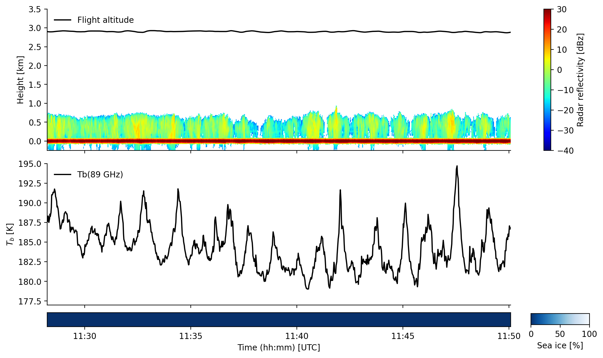
The flight section during ACLOUD RF05 is flown at about 3 km altitude in west-east direction during a cold-air outbreak event perpendicular to the wind field. Clearly one can identify the roll-cloud structure in the radar reflectivity and the 89 GHz brightness temperature.

%matplotlib inline
import matplotlib.pyplot as plt
import matplotlib.dates as mdates
import numpy as np
plt.style.use("../../mplstyle/book")

fig, (ax1, ax2, ax3) = plt.subplots(3, 1, sharex=True, gridspec_kw=dict(height_ratios=(1, 1, 0.1)))

# 1st: plot flight altitude and radar reflectivity
ax1.plot(ds_mirac_a_sel.time, ds_mirac_a_sel.alt*1e-3, label='Flight altitude', color='k')

im = ax1.pcolormesh(ds_mirac_a_sel.time, ds_mirac_a_sel.height*1e-3, 10*np.log10(ds_mirac_a_sel.Ze).T, vmin=-40, vmax=30, cmap='jet', shading='nearest')
fig.colorbar(im, ax=ax1, label='Radar reflectivity [dBz]')
ax1.set_ylim(-0.25, 3.5)
ax1.set_ylabel('Height [km]')
ax1.legend(frameon=False, loc='upper left')

# 2nd: plot 89 GHz TB
ax2.plot(ds_mirac_a_sel.time, ds_mirac_a_sel.tb, label='Tb(89 GHz)', color='k')
ax2.set_ylim(177, 195)
ax2.set_ylabel('$T_b$ [K]')
#ax2.set_xlabel('Time (hh:mm) [UTC]')
ax2.legend(frameon=False, loc='upper left')

#ax2.xaxis.set_major_formatter(mdates.DateFormatter('%H:%M'))

# plot AMSR2 sea ice concentration
im = ax3.pcolormesh(ds_sea_ice.time,
               np.array([0, 1]),
               np.array([ds_sea_ice.sic,ds_sea_ice.sic]), cmap='Blues_r', vmin=0, vmax=100,
               shading='auto')
cax = fig.add_axes([0.9, 0.085, 0.1, ax3.get_position().height])
fig.colorbar(im, cax=cax, orientation='horizontal', label='Sea ice [%]')
ax3.tick_params(axis='y', labelleft=False, left=False)
ax3.spines[:].set_visible(True)
ax3.xaxis.set_major_formatter(mdates.DateFormatter('%H:%M'))
ax3.set_xlabel('Time (hh:mm) [UTC]')

plt.show()

LWP

list(cat['ACLOUD']['P5']['MiRAC-A_LWP'])

['ACLOUD_P5_RF05',
 'ACLOUD_P5_RF06',
 'ACLOUD_P5_RF07',
 'ACLOUD_P5_RF11',
 'ACLOUD_P5_RF14',
 'ACLOUD_P5_RF15',
 'ACLOUD_P5_RF16',
 'ACLOUD_P5_RF18',
 'ACLOUD_P5_RF19',
 'ACLOUD_P5_RF20',
 'ACLOUD_P5_RF21',
 'ACLOUD_P5_RF22']

ds_lwp = cat['ACLOUD']['P5']['MiRAC-A_LWP']['ACLOUD_P5_RF05'].to_dask()

ds_lwp

<xarray.Dataset>
Dimensions:      (time: 11765)
Coordinates:
  * time         (time) datetime64[ns] 2017-05-25T08:18:18 ... 2017-05-25T12:...
    lat          (time) float64 78.25 78.25 78.25 78.25 ... 78.29 78.29 78.29
    lon          (time) float64 15.42 15.41 15.41 15.41 ... 15.05 15.05 15.05
Data variables:
    trajectory   |S1 b''
    alt          (time) float32 150.0 158.2 166.0 180.7 ... 855.4 851.0 846.5
    status_flag  (time) int32 48 48 48 48 48 48 48 48 ... 32 32 32 32 32 32 32
    lwp          (time) float32 nan nan nan nan nan nan ... nan nan nan nan nan
Attributes: (12/14)
    institution:  Institute for Geophysics and Meteorology, University of Col...
    contact:      l.kliesch@uni-koeln.de, mario.mech@uni-koeln.de
    source:       Kliesch and Mech (2019, doi: https://doi.org/10.1594/PANGAE...
    Conventions:  CF-1.7
    title:        LWP retrieval of MiRAC on Polar 5
    variable:     liquid water path (LWP)
    ...           ...
    campaign:     ACLOUD: Arctic CLoud Observations Using airborne measuremen...
    keywords:     LWP, MiRAC, ACLOUD, Polar 5
    featureType:  trajectory
    history:      created: 2021-05-27
    author:       Leif-Leonard Kliesch
    summary:      LWP is retrieved nadir over sea-ice-free ocean from the 89 ...

xarray.Dataset

• Dimensions:
  • time: 11765
• Coordinates: (3)
  • time
    (time)
    datetime64[ns]
    2017-05-25T08:18:18 ... 2017-05-...

    long_name :

    unixtime

    standard_name :

    time

    array(['2017-05-25T08:18:18.000000000', '2017-05-25T08:18:19.000000000',
           '2017-05-25T08:18:20.000000000', ..., '2017-05-25T12:40:20.000000000',
           '2017-05-25T12:40:21.000000000', '2017-05-25T12:40:22.000000000'],
          dtype='datetime64[ns]')

  • lat
    (time)
    float64
    ...

    units :

    degree_north

    standard_name :

    latitude

    valid_range :

    [-90. 90.]

    long_name :

    latitude of platform position

    array([78.249123, 78.249268, 78.249413, ..., 78.294189, 78.294067, 78.293945])

  • lon
    (time)
    float64
    ...

    units :

    degree_east

    standard_name :

    longitude

    valid_range :

    [-180. 180.]

    long_name :

    longitude of platform position

    array([15.416362, 15.414106, 15.41187 , ..., 15.046572, 15.049372, 15.052175])

• Data variables: (4)
  • trajectory
    ()
    |S1
    ...

    long_name :

    trajectory identifier

    cf_role :

    trajectory_id

    array(b'', dtype='|S1')

  • alt
    (time)
    float32
    ...

    units :

    m

    long_name :

    altitude above mean sea level

    standard_name :

    altitude

    positive :

    up

    description :

    platform altitude

    array([150.03773, 158.23862, 165.955  , ..., 855.40424, 850.99915, 846.541  ],
          dtype=float32)

  • status_flag
    (time)
    int32
    ...

    standard_name :

    status_flag

    flag_values :

    [ 0 2 4 8 16 32]

    description :

    LWP retrieval is valid over sea ice free ocean surface and for optimal platfrom positioning and altitude

    comment :

    unvalid_conditions_for_retrieval means surface type dominated by sea ice or land or sensor problems; status_flag values > 0 should be avoided.

    flag_meanings :

    quality_good unvalid_conditions_for_retrieval sea_ice_floes platform_roll_angle_larger_5deg platform_pitch_angle_larger_5deg flight_altitude_below_2800_m

    array([48, 48, 48, ..., 32, 32, 32], dtype=int32)

  • lwp
    (time)
    float32
    ...

    units :

    kg m-2

    long_name :

    retrieved column integrated cloud liquid water path (lwp)

    standard_name :

    atmosphere_mass_content_of_cloud_liquid_water

    description :

    Nadir lwp retrieved from 89 GHz measuring at 25deg inclination. The lwp retrieval techique is described in Donoso et al. (2020, https://doi.org/10.5194/acp-20-5487-2020).

    comment :

    estimated uncertainty of about 0.020 kg m-2

    array([nan, nan, nan, ..., nan, nan, nan], dtype=float32)

• Attributes: (14)

  institution :

  Institute for Geophysics and Meteorology, University of Cologne

  contact :

  l.kliesch@uni-koeln.de, mario.mech@uni-koeln.de

  source :

  Kliesch and Mech (2019, doi: https://doi.org/10.1594/PANGAEA.899565)

  Conventions :

  CF-1.7

  title :

  LWP retrieval of MiRAC on Polar 5

  variable :

  liquid water path (LWP)

  platform :

  Polar 5

  instrument :

  MiRAC: Microwave Radar/radiometer for Arctic Clouds (Mech et al. 2019, https://doi.org/10.5194/amt-12-5019-2019)

  campaign :

  ACLOUD: Arctic CLoud Observations Using airborne measurements during polar Day

  keywords :

  LWP, MiRAC, ACLOUD, Polar 5

  featureType :

  trajectory

  history :

  created: 2021-05-27

  author :

  Leif-Leonard Kliesch

  summary :

  LWP is retrieved nadir over sea-ice-free ocean from the 89 GHz channel of MiRAC, which is inclined by 25deg backwards from nadir and flight direction of Polar 5. Polar 5, the research aircraft of the Alfred Wegener Institute for polar and ocean research (AWI), flew during the ACLOUD campaign in summer 2017 conducted from Longyearbyen/Svalbard (Wendisch et al. 2018, https://doi.org/10.1175/BAMS-D-18-0072.1).

fig, (ax1, ax2) = plt.subplots(2, 1, sharex=True)

# 1st: plot 89 GHz TB
ax1.plot(ds_mirac_a.time, ds_mirac_a.tb, label='Tb(89 GHz)', color='k')
ax1.set_ylim(160, 250)
ax1.set_ylabel('$T_b$ [K]')
ax1.set_xlabel('Time (hh:mm) [UTC]')
ax1.legend(frameon=False, loc='upper left')

# 2nd: plot 89 GHz TB
ax2.plot(ds_lwp.time, ds_lwp.lwp, label='LWP', color='b')
#ax2.set_ylim(177, 195)
ax2.set_ylabel('LWP [g/m^2]')
ax2.set_xlabel('Time (hh:mm) [UTC]')
ax2.legend(frameon=False, loc='upper left')

ax2.xaxis.set_major_formatter(mdates.DateFormatter('%H:%M'))

plt.show()