Fish-eye camera#

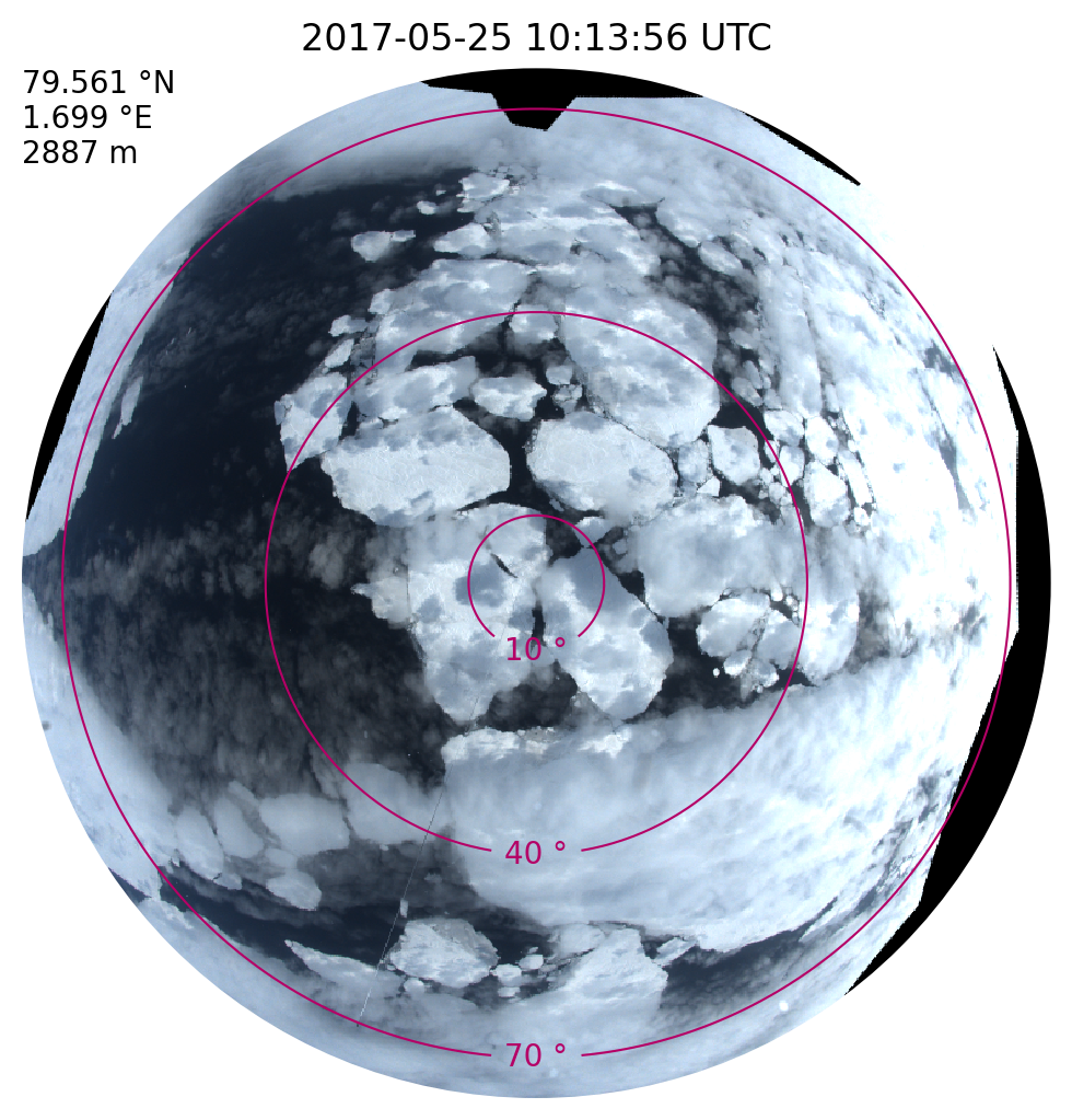
A downward-looking commercial digital camera equipped with a 180°-fisheye lens was installed on the aircraft Polar 5. Images of the Arctic surface and clouds were taken every 4-6 seconds. The data set provides rectified fields of calibrated radiances along the flight track for the three spectral bands (red, green, and blue). The full dataset is available on PANGAEA for ACLOUD, AFLUX and MOSAiC-ACA. In the next sections, the data is loaded from the PANGAEA database and a cloudy scene over sea ice is plotted.

Data access#

To analyse the data they first have to be loaded by importing the (AC)³airborne meta data catalogue. To do so the ac3airborne package has to be installed. More information on how to do that and about the catalog can be found here.

Get data#

import ac3airborne

cat = ac3airborne.get_intake_catalog()

datasets = []
for campaign in ['ACLOUD', 'AFLUX', 'MOSAiC-ACA']:
    datasets.extend(list(cat[campaign]['P5']['FISH_EYE_CAMERA']))
datasets

['ACLOUD_P5_RF05',
 'ACLOUD_P5_RF06',
 'ACLOUD_P5_RF07',
 'ACLOUD_P5_RF08',
 'ACLOUD_P5_RF10',
 'ACLOUD_P5_RF11',
 'ACLOUD_P5_RF13',
 'ACLOUD_P5_RF14',
 'ACLOUD_P5_RF15',
 'ACLOUD_P5_RF16',
 'ACLOUD_P5_RF17',
 'ACLOUD_P5_RF18',
 'ACLOUD_P5_RF19',
 'ACLOUD_P5_RF20',
 'ACLOUD_P5_RF21',
 'ACLOUD_P5_RF22',
 'ACLOUD_P5_RF23',
 'ACLOUD_P5_RF25',
 'AFLUX_P5_RF03',
 'AFLUX_P5_RF04',
 'AFLUX_P5_RF05',
 'AFLUX_P5_RF06',
 'AFLUX_P5_RF07',
 'AFLUX_P5_RF08',
 'AFLUX_P5_RF09',
 'AFLUX_P5_RF10',
 'AFLUX_P5_RF11',
 'AFLUX_P5_RF12',
 'AFLUX_P5_RF13',
 'AFLUX_P5_RF14',
 'AFLUX_P5_RF15',
 'MOSAiC-ACA_P5_RF04',
 'MOSAiC-ACA_P5_RF05',
 'MOSAiC-ACA_P5_RF06',
 'MOSAiC-ACA_P5_RF07',
 'MOSAiC-ACA_P5_RF08',
 'MOSAiC-ACA_P5_RF09',
 'MOSAiC-ACA_P5_RF10',
 'MOSAiC-ACA_P5_RF11']

Note

Have a look at the attributes of the xarray dataset ds_cam for all relevant information on the dataset, such as author, contact, or citation information.

The dataset includes the red, green and blue radiances (radiance_red, radiance_green, radiance_blue), the camera’s zenith and azimuth angles (vza, vaa), and information on the aircraft’s flight altitude (altitude) and position (latitude, longitude).

Next, the time is converted from dec UTC to datetime:

import datetime
import numpy as np

def convert_time(ds):
    """
    Convert time 
    """

    date = datetime.datetime.strptime(ds.attrs['Comment'], 'Date %Y-%m-%d')
    time = np.array([(date + datetime.timedelta(hours=h)).replace(microsecond=0) for h in ds.time.values.astype('float')])
    
    ds['time'] = (('dim_t'), time)
    
    return ds

print(ds_cam.time.dtype)
ds_cam = convert_time(ds_cam)
print(ds_cam.time.dtype)

float32
datetime64[ns]

Plots#

%matplotlib inline
import matplotlib.pyplot as plt
from matplotlib import patches
plt.style.use("../../mplstyle/book")

def scaling(x, a, b, x_min=None, x_max=None):
    """    
    Scale values x in new range from a to b
    """
    
    if x_min is None:
        x_min = np.min(x)

    if x_max is None:
        x_max = np.max(x)
        
    x_scaled = a + (x-x_min) * (b-a) / (x_max-x_min)
    
    return x_scaled

# select timestep
t = 117

fig, ax = plt.subplots(1, 1, figsize=(5, 5), constrained_layout=True)

# 1: convert radiances to RGB image
rgb = np.stack([ds_cam[c].sel(dim_t=t) for c in ['radiance_red', 'radiance_green', 'radiance_blue']])

# scale radiances between 0 and 255, with 255 = 95th percentile of RGB radiances
max_radiance = np.percentile(rgb, 95)
rgb = scaling(x=rgb.astype('float64'), 
              a=0, 
              b=255, 
              x_min=0, 
              x_max=max_radiance)
rgb = np.round(rgb, 0).astype('int')
rgb = rgb.transpose(1, 2, 0)
# set values that exceed the 95 percentile
rgb[rgb > 255] = 255
im = ax.imshow(rgb, interpolation='nearest')

# zoom into center of image
center = 450
radius = 380
patch = patches.Circle((center, center), radius=radius, fc='none')
ax.add_patch(patch)
im.set_clip_path(patch)

# set axis limits: image origin is upper left corner
ax.set_xlim(center-radius, center+radius)
ax.set_ylim(center+radius, center-radius)

# 2: show viewing angle grid
ct_vza = ax.contour(ds_cam.dim_x, ds_cam.dim_y, ds_cam.vza*1e-2, levels=np.array([10, 40, 70]), colors='#B50066', linestyles='-', linewidths=0.75)
ax.clabel(ct_vza, fmt='%1.0f °', manual=[(center, 490), (center, 640), (center, 800)])

# 3: add meta information
alt = ds_cam.altitude.sel(dim_t=t).values.item()
time = datetime.datetime.utcfromtimestamp((ds_cam.time.sel(dim_t=t).values - np.datetime64('1970-01-01 00:00:00')) / np.timedelta64(1, 's'))
lon = ds_cam.longitude.sel(dim_t=t).values.item()
lat = ds_cam.latitude.sel(dim_t=t).values.item()

txt = '{} °N\n{} °E\n{} m'.format(np.round(lat, 3), np.round(lon, 3), int(np.round(alt, 0)))
ax.annotate(txt, xy=(center-radius, center-radius), xycoords='data', ha='left', va='top')

time_txt = time.strftime('%Y-%m-%d %H:%M:%S UTC')
ax.set_title(time_txt)

ax.axis('off')

plt.show()

how_to_ac3airborne

Fish-eye camera

Contents

Fish-eye camera#

Data access#

Get data#

Plots#